Week 6 - CHT Analysis on a Graphics card

Conjugate heat transfer analysis on a graphics card

Objectives:

To Run the simulation by varying the velocity from 1m/sec to 5m/sec for at least 3 velocities and discuss the results.

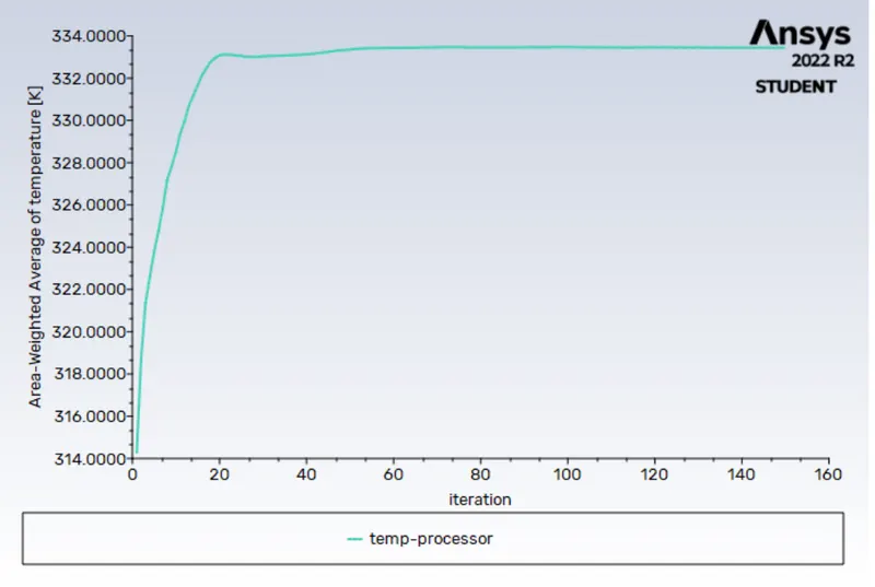
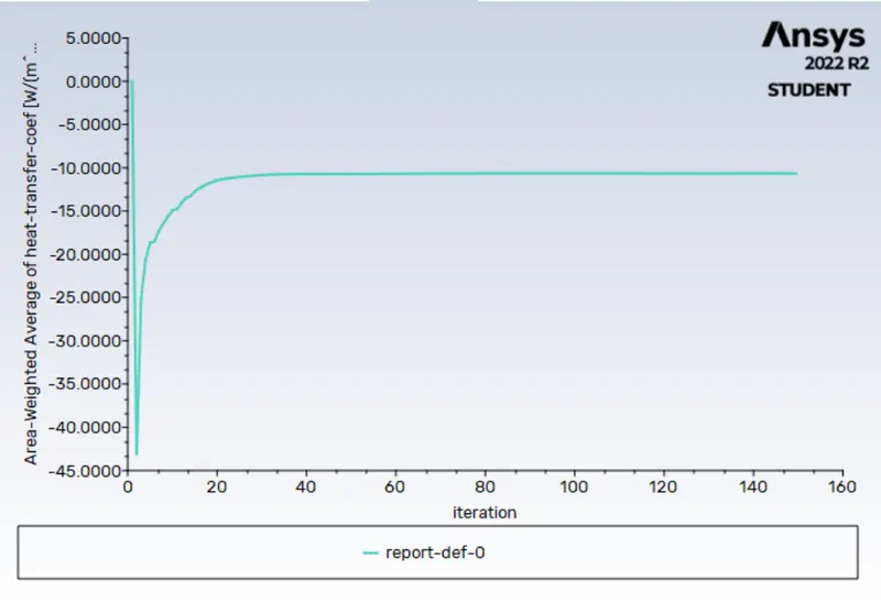
To Find out the maximum temperature and heat transfer coefficient attained by the processor.

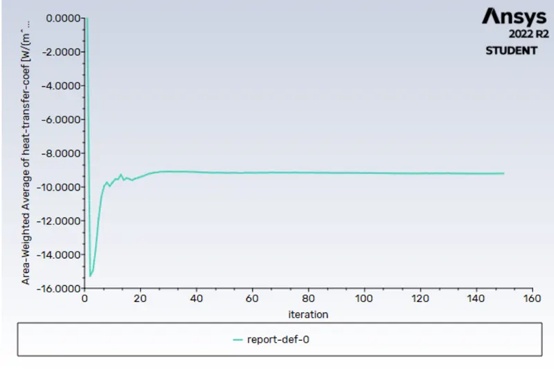
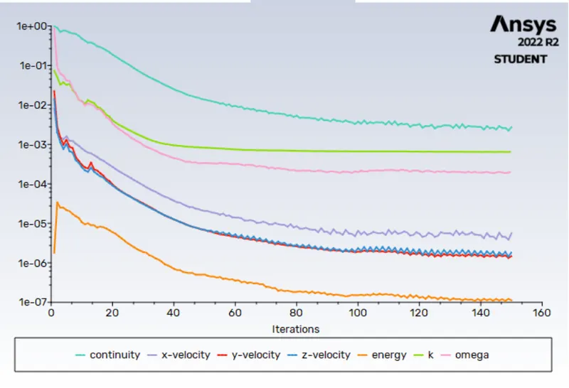
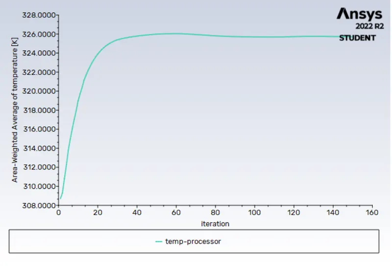
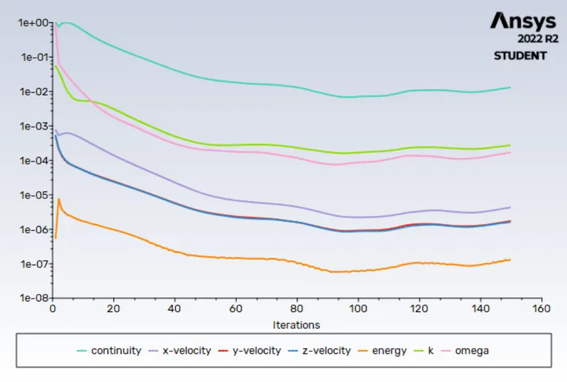
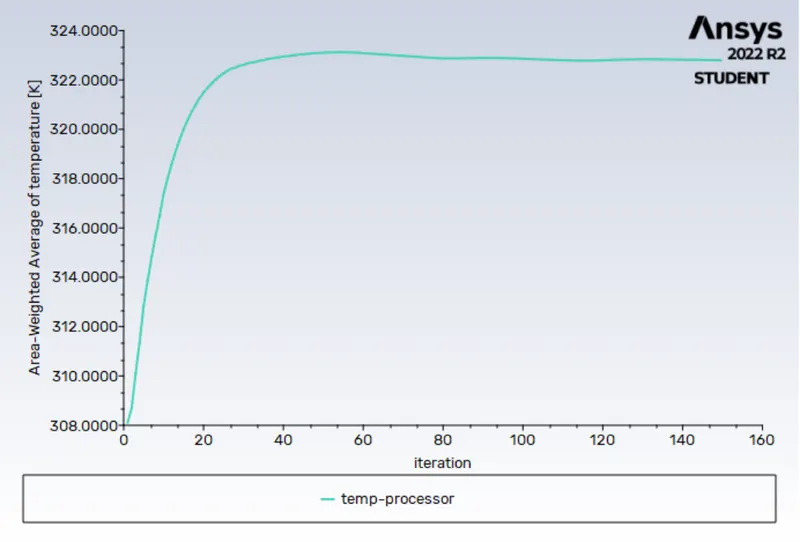
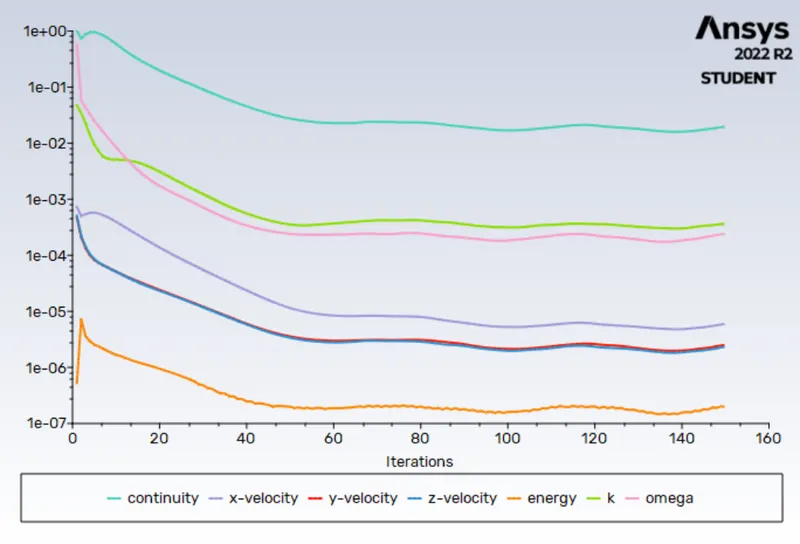
To Prove that the simulation has achieved convergence with appropriate images and plots.

To Identify potential hotspots on the model.

Conjugate heat transfer:

Conjugate Heat Transfer analysis allows for the simulation of heat transfer between solid and fluid domains by exchanging thermal energy at the interfaces between them and transported via conduction within solids and additionally via convection within fluid domains.

Conjugate heat transfer analysis can accurately predict heat transfer by simultaneous solving all the relevant solid and flow field heat transfer processes. Conjugate heat transfer corresponds with the combination of heat transfer in solids and heat transfer in fluids.

In solids, conduction often dominates whereas in fluids, convection usually dominates. Conjugate heat transfer is observed in many situations for example: conduction through solids, free and forced convection in the gases/fluids and thermal radiation.

The three main modes of heat transfer:

‐ Conduction is heat transfer that occurs when a temperature difference exists across a stationary medium.

‐ Convection is the heat transfer between a surface and a moving fluid when there is a temperature difference between the two.

‐ Radiation (thermal radiation) is the emission of energy in the form of electromagnetic waves. In the absence of an intervening medium, there is net heat transfer by radiation between two surfaces at different temperatures.

Procedure

For solving it we follow the below procedure:

1)Geometry setup

2)Meshing

3) Problem setup

4)Solving

5)Post processing

Then we calculate the wall/surface heat transfer coefficient on the internal solid surface & show the velocity & temperature contours in appropriate areas.

Geometry setup:

1. Use Space claim to edit the geometry of the downloaded model of the graphics card which is in the enclosure.
2. Click on share prep to view any edges in interference so that conformal mesh can be achieved between different components.
3. Share topology has to be enabled between the different components so that necessary information can be shared between different zones of the mesh.

Given model

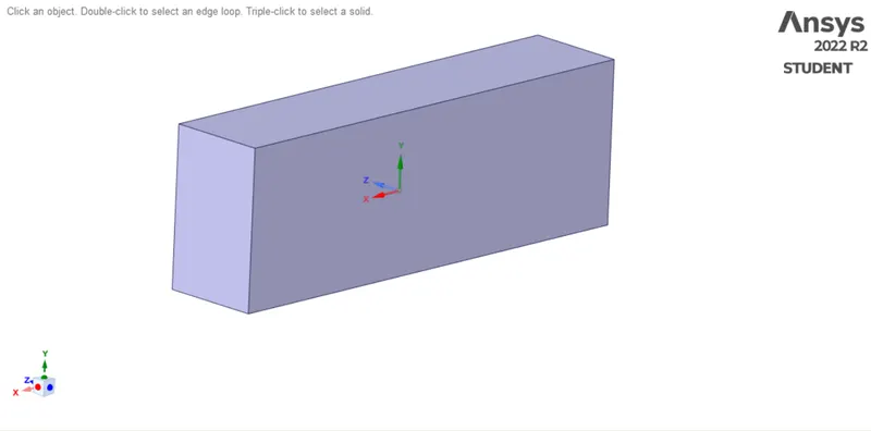
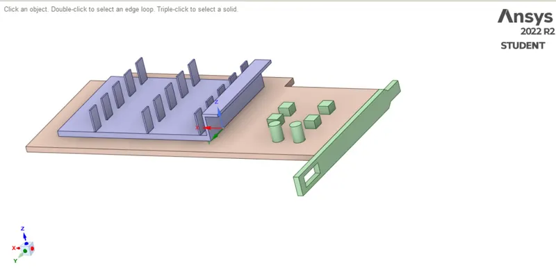
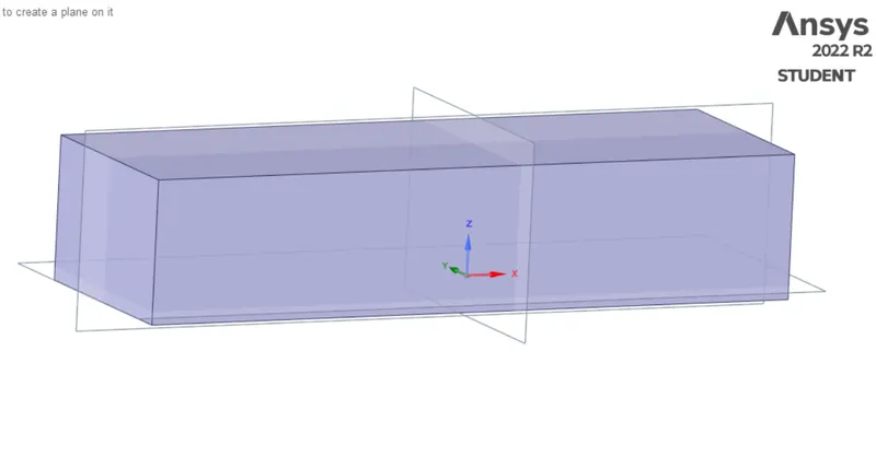
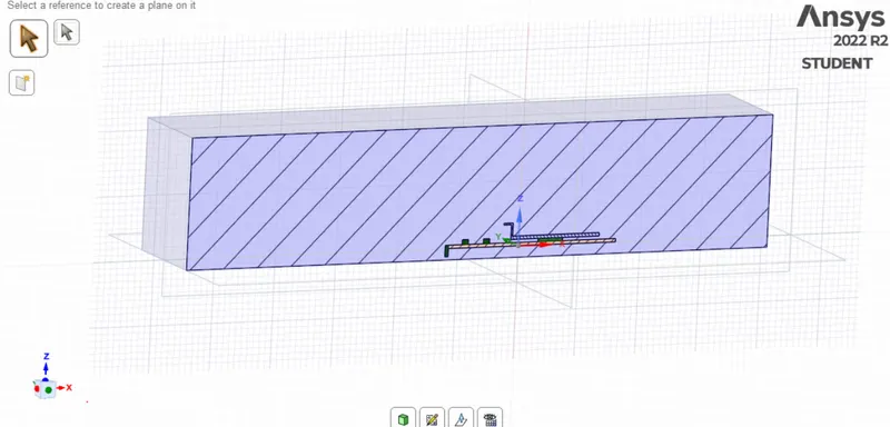
section views of graphic card

Mesh setup:

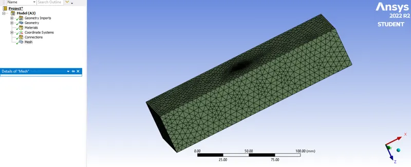
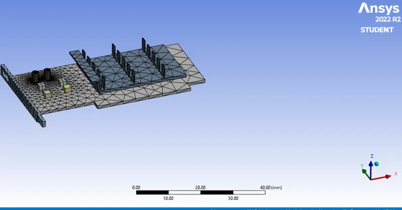
1. Before generating a base mesh, let's name the different components of the graphic card so it is easier to find them while setting up fluent.
2. Enclosure, inlet, outlet, Pcb, processor and fins are basic name selections which will help us in the simulation.
3. Click generate mesh to create a base mesh which is 10mm.
4. After creating the mesh, exit Mesh setup to simulate in fluent.

Fluent setup:

Right click on the setup and click edit select double precision and solver as 4 for better results. In this problem we use steady state solver. For heat transfer problems we need to enable energy equations.

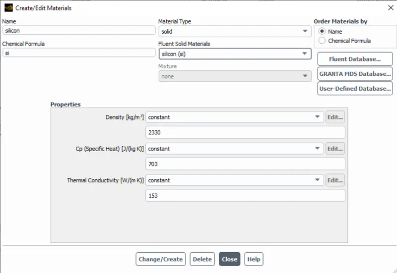
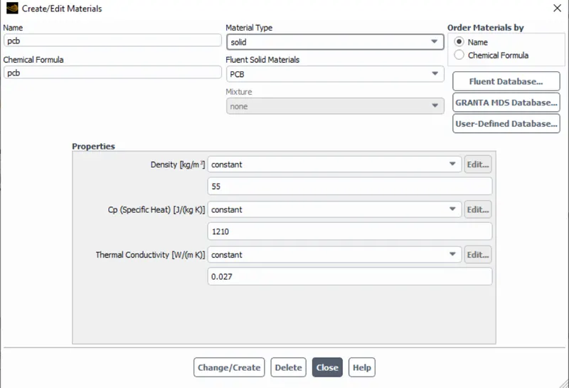
Materials used

here we have given some conditions for the PCB, processor, and fins here we have used silicon, aluminum and the values are taken from the data book

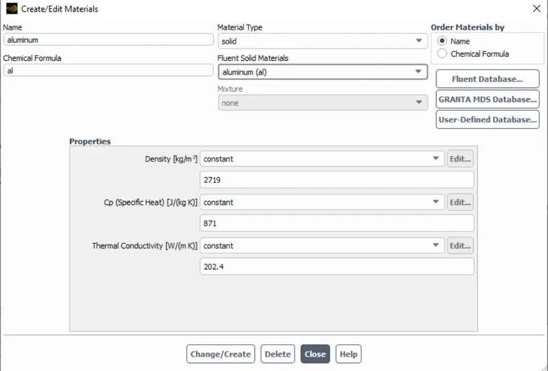
Cell zone conditions

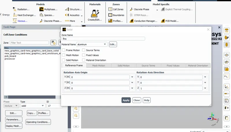
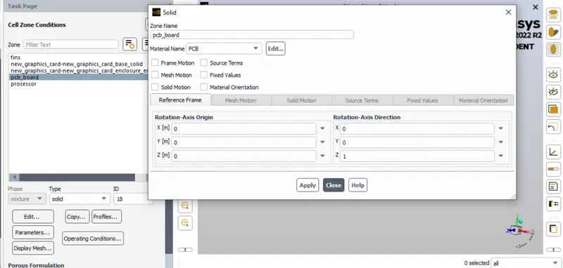
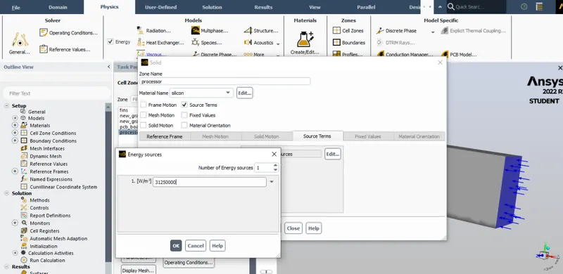
Here we are enabling the source terms and giving the input for the processor

Boundary conditions: We will basically give our boundary conditions here such as inlet velocity and outlet conditions.

we give,

Case 1

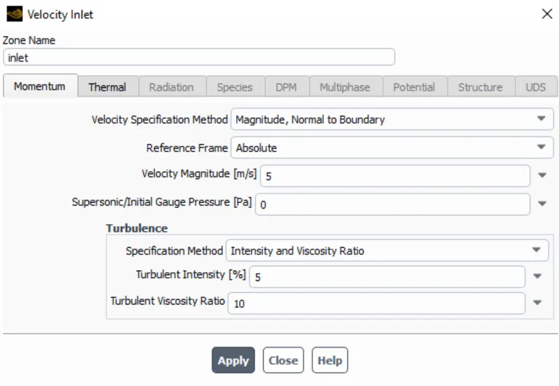
Inlet velocity: 3m/s

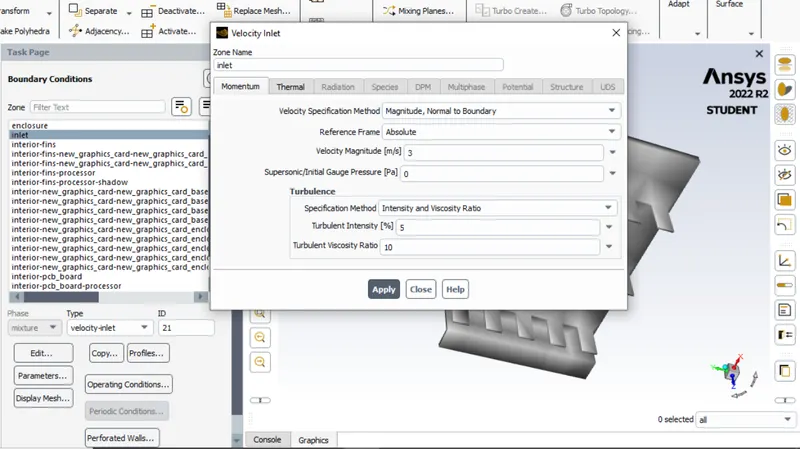
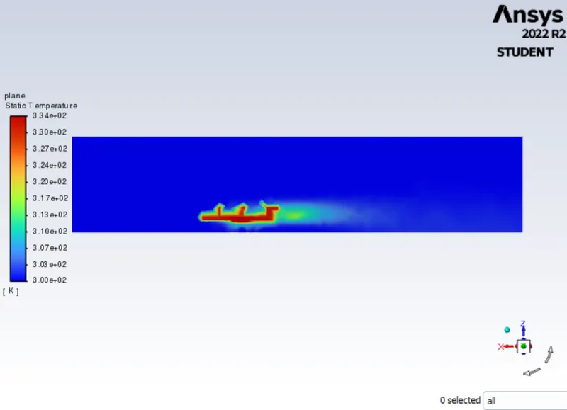
Now we are almost ready to run the simulation, but as the solution is being solved, we want to monitor different flow quantities while the solution is being generated. But before that we have to initialize the domain. Click on run calculation for 150 iterations. Then we can see that in the residual plot that residuals drop and reach a steady state after 100 iterations. Then let us post the process results. After running the calculations, look at the console to see if the given values are enough to converge. And select >> results in left side tool bar click on the contours option to create the contour plot for the temperature, velocity, heat transfer coefficient for better understanding. For better viewing the temperature inside the model select results>> create >> plane >> select the plane that needed for better visualizing the contours.

Results

Processor temperature

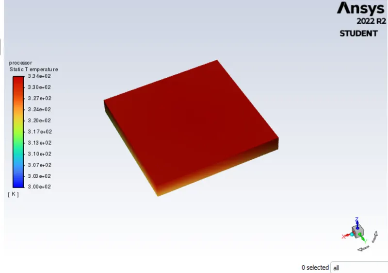
PLANE view

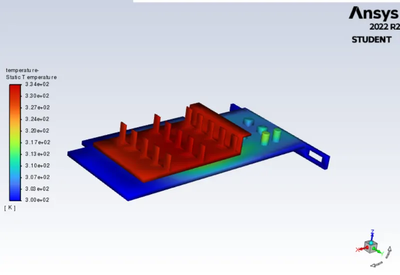
Graphic card Temperature

Heat transfer Coeff plot

Temperature plot

Case 2

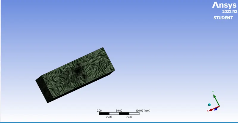
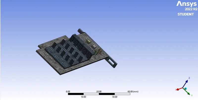
Refined Mesh

Here we are giving different mesh sizes for each element

Inlet, Enclosure, outlet = 3mm

Pcb, fins = 1mm

Processor = 1mm

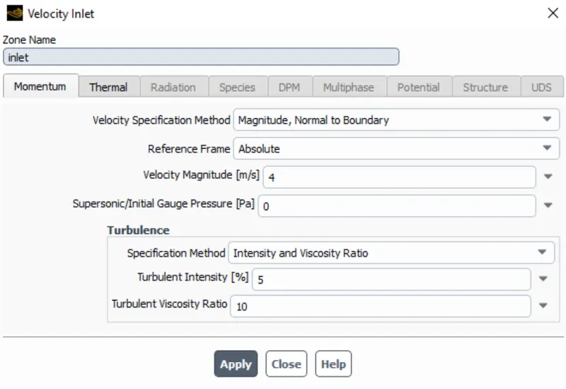
Inlet velocity- 4m/s

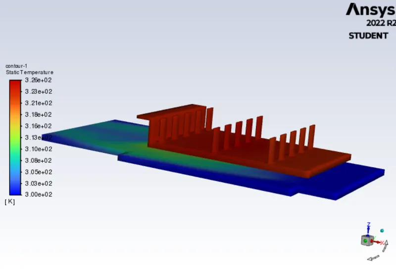
results

Temperature of graphics card

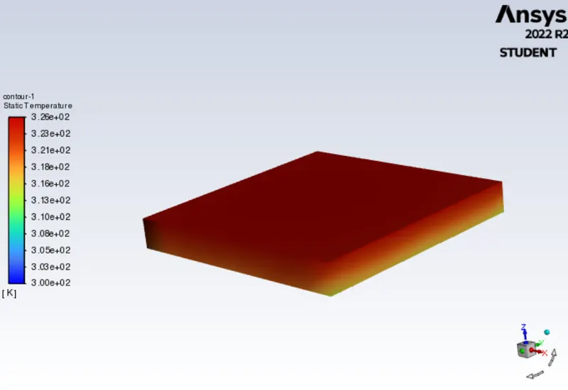
Temperature of processor

Heat transfer Coeff of processor

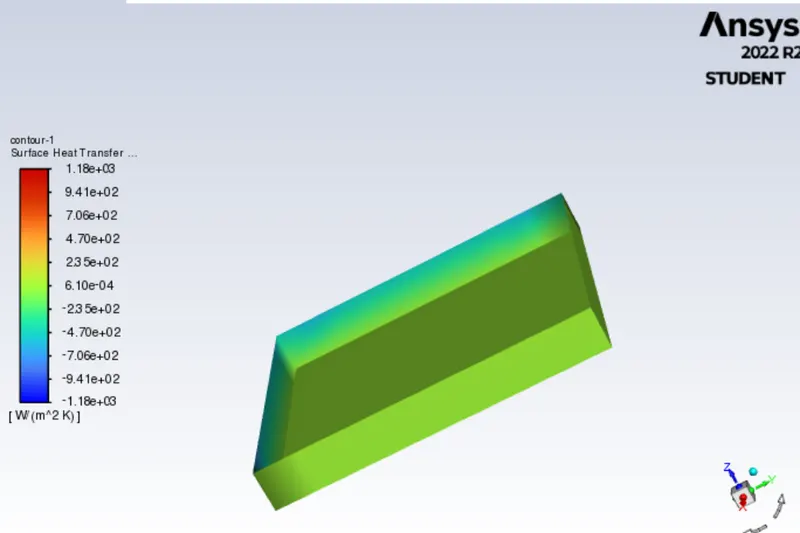
Temperature plot

Heat transfer Coeff plot

Case 3

Refined mesh

Here we are giving different mesh sizes for each element

Inlet, Enclosure, outlet = 3mm

Pcb, fins, Processor = 1mm

Inlet velocity- 5m/s

Results

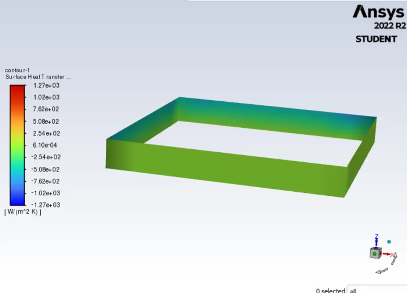
Heat transfer Coeff of processor

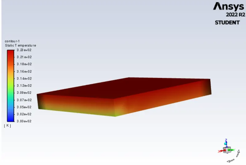
Temperature of processor and graphic card

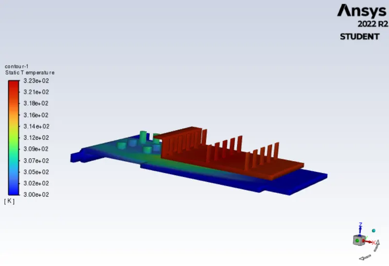
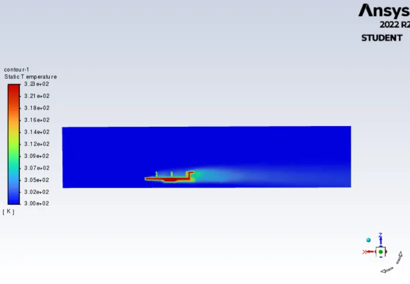
Temperature plot

Heat transfer Coeff plot

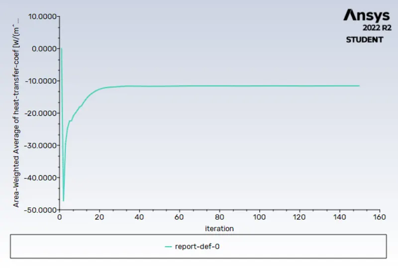
Case velocity HTC Max temperature [k]

Case 1 3m/s -12.2092 1192

Case 2 4m/s -14.7764 1092

Case 3 5m/s -16.9939 902

Conclusion

A converged solution for the given sets of input was observed on the basis of repetitive plots in the Residual plot. The processor acted as a source of heat input and thus one of the hotspots for such study

With an increase in velocity, we saw a considerable drop in temperature and a substantial rise in heat transfer coefficient which shows that high-velocity air can be an effective mode of heat dissipation in graphics card

From the temperature distribution, we can see hotspots in the fin and base near the surface that is in contact with the processor. Based on the thermal conductivity of the material this temperature is distributed accordingly amongst the components. We see a few high-temperature zones on fin away from processor depicting their high susceptibility to heat due to their geometry.

Also, the difference in baseline and refined mesh is considerable and thus we can conclude that more refined mesh provides a better solution and can be used in optimizing the design for such applications. From the residual plot, the change in the gradients is very small with which we can conclude that the solution has converged.

From the temperature plot of the coarse mesh, the high-temperature points are found at fins, processor, and base area near the processor. As the wall heat transfer coefficient is a wall phenomenon and fins dissipate a large amount of heat which results in higher heat transfer co-efficient but the coarse mesh heat transfer for fins and other components in the graphics card has the same values. Hence refinement of mesh is done for fins and base of the fin and base of the graphic card in order to calculate the wall heat transfer coefficient at the fins and base.

The high-temperature regions are found at the center of the fins, base, and the processor walls. With further iterations, the temperature is distributed to other regions in the graphics card in the direction of the inlet airflow. Conduction occurs where there is a contact region between the solids, in this case it is between processor and fins and processor and base. Convection occurs when the heat generated in the components of the graphic card is removed by the inlet airflow. The maximum temperature in the components is inversely proportional to the inlet airflow velocity. With the increase in the airflow velocity, the heat removal process by convection is faster. And also, recirculation of air (vortex) at appropriate places will increase the heat transfer efficiencies hence greater amount of heat is removed by convection.