CHT Analysis on a Graphics card

Aim:-

• Perform a steady-state conjugated heat transfer analysis on a model of a graphics card.
• Select the appropriate materials for the simulation.
• Mesh the geometry with a desirable combination and Explain the mesh setting used on this model.
• Simulate by varying the velocity from 1m/s to 5m/s for at least 3 velocities and discuss the results.
• Find out the maximum temperature and heat transfer coefficient attained by the processor.
• Prove that the simulation has achieved convergence with appropriate images and plots.
• Identify potential hot spots on the model.

Objectives:-

• Import graphics card model in the space claim and active share topology.
• Mesh the model using proper inflation layer and face sizing.
• Open fluent setup and perform steady-state conjugated heat transfer simulation on meshed model.
• Prove that the simulation has achieved convergence with appropriate images and plots.
• Check the mesh independence of the model by performing the same simulation with different densities of mesh.
• Try simulating solution using different velocity between range 1m/s to 5m/s
• Find out the maximum temperature and heat transfer coefficient attained by the processor.
• Identify potential hot spots on the model.

Conjugate Heat Transfer Analysis

The Conjugate Heat Transfer (CHT) analysis type allows for the simulation of heat transfer between solid and fluid domain by exchanging thermal energy at the interface between them.

In solids, conduction often dominates whereas, in fluids, convection usually dominates.

The physics of conjugated heat transfer is common in many engineering applications, including heat exchangers, HVAC, and electronic components design.

Workbench Setup

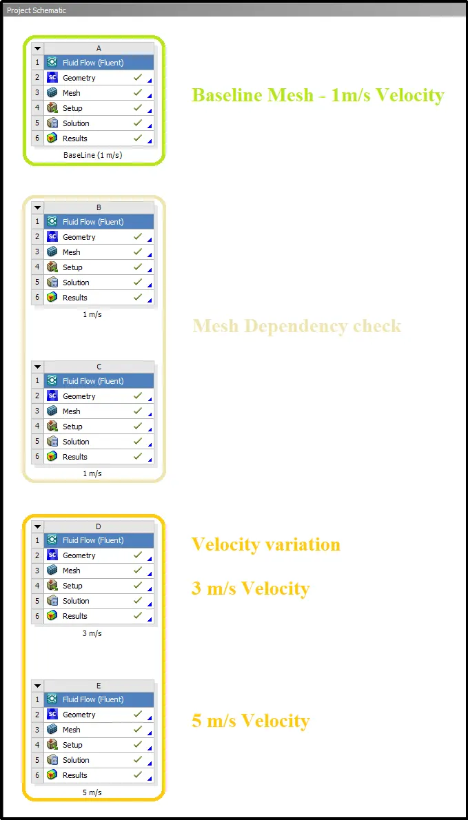
In this study, a total of 5 simulations was simulated. The first one was the baseline simulation for getting a rough idea and results for the further final simulations.

The next two simulations were performed to check the mesh dependency of the problem setup.

The last two cases were performed to run simulations for different velocities to get study how final results affect by velocity variation.

Geometry Checkup:-

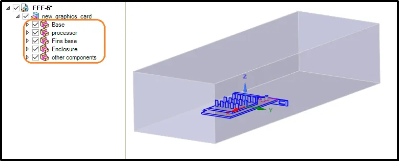
At the starting of the simulation process, the made-up (Rough) geometry of the graphics card which also already includes encloser was imported into the Space Claim. The various components involved in the geometry are highlighted with the orange rectangular boundary line which includes the base (circuit board), Graphics card processor, Fins attached to the processor, and other components.

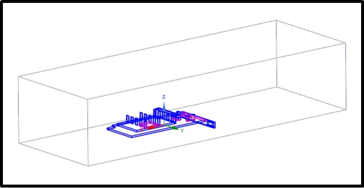
The geometry and flow domain consists of a flat circuit board with a heat-generating electronic processor chip and some other components connected to it. Heat is conducted through the source (processor), the board mounted on it and the fins attached to the processor. A stream of air flows over the fins, processor, and board, causing simultaneous cooling of the solid components and heating of the airstream due to convection. Thermal energy is also transported due to the complex flow field.

Meshing:-

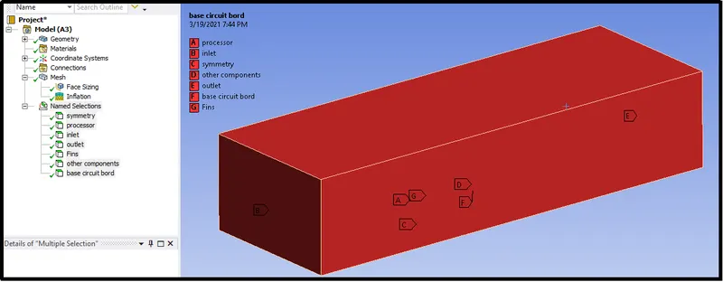
The first step into meshing should be to provide a name to each surface and component which was given as depicted in the below picture.

Baseline mesh (For First simulation baseline mesh was used)

In baseline meshing, two inflation layers with a total thickness of 0.4mm were used to get an idea of the Y+plus value. With the reference of this Y+ value inflation layer for final simulation mesh is considered.

It is difficult for this simulation to calculate the Reynolds number for this problem as it is difficult to calculate the characteristic length of the circuit and fins. But we know that for the turbulence model we need y+ less than 5 to get desirable results. Therefore it is good practice to run baseline simulation with rough first layer thickness.

Here if we considered total thickness as 0.4 with 2 layers, therefore the first layer thickness we got is

`dY = (Tt)/(Gr^(n-1))`

n = number of layers

Gr = growth rate

Tt = total thickness

dY = first layer thickness

First Layer thickness

`dY = 0.4/(1.2^((2-1))`

`dY = 0.33334`

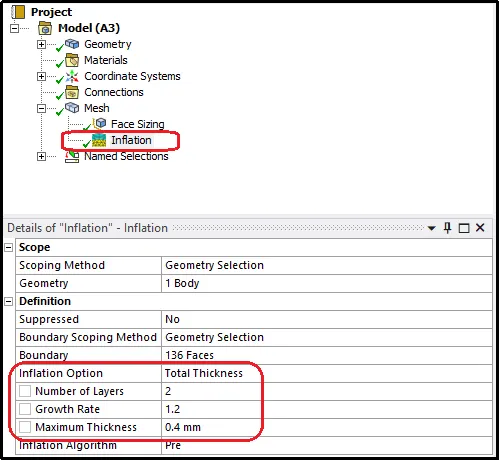
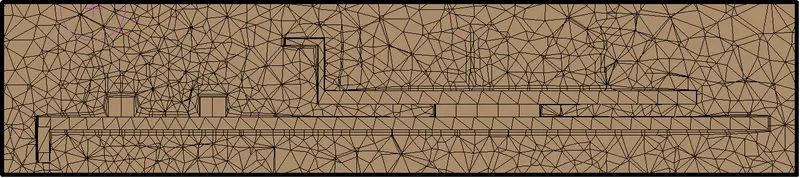
Overview of the mesh after implementing the above settings of inflation layers.

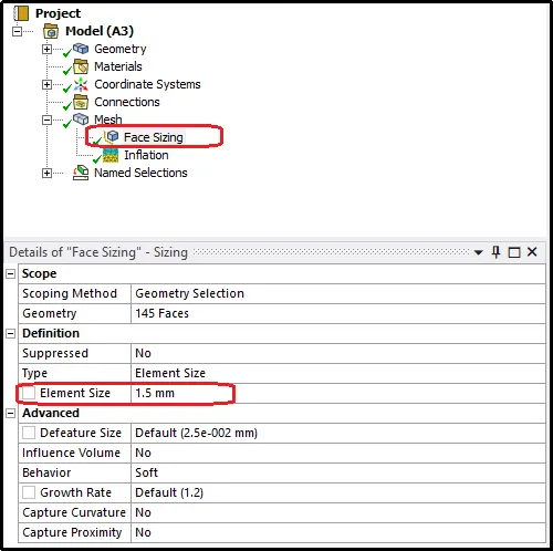
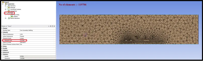
Next, to refine the mesh near the graphics card circuit area, actually where the accuracy of the simulation is required, face sizing of 1.5mm was used.

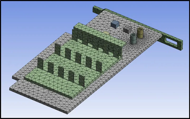
Generation of mesh over a graphics card circuit will show the following results after the use of the above element size on the faces.

Mesh size for other regions was considered as 5mm. The overall mesh growth rate was taken as the default value which is 1.2.

Fluent Setup

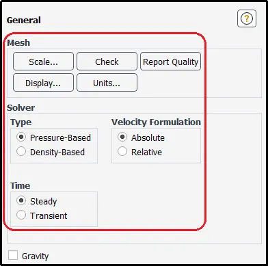
In the Fluent settings, the type of solver is used as a pressure base. Velocity formulation was set to absolute and problem simulated as considering steady-state simulation.

In this particular simulation, the temperature must be calculated so the energy equation needs to be enabled.

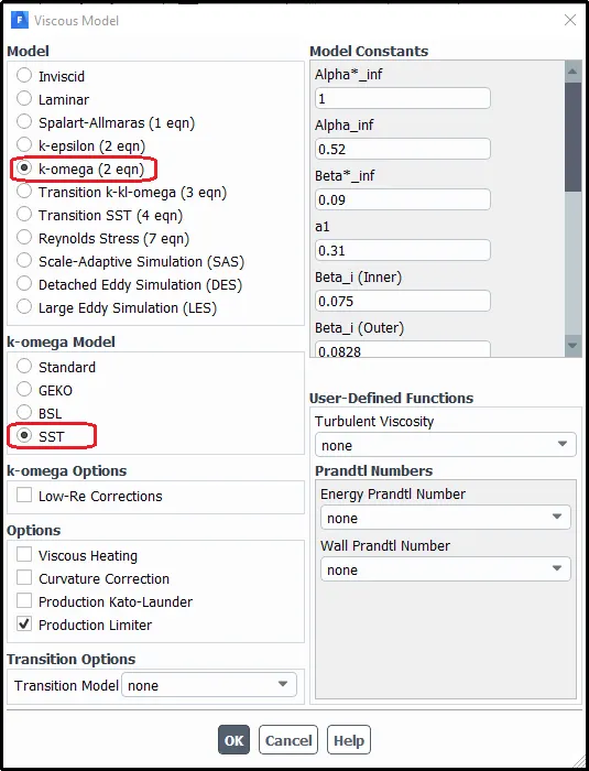
For this simulation, the k-omega turbulent model is considered which is best used for near-wall treatment. This is vital for this simulation as we expect the heat transfer coefficient calculated on the surfaces.

From the K-omega model, SST was selected as it provides a better prediction of flow separation than most RANS models and also accounts for its good behavior in adverse pressure gradients. It has the ability to account for the transport of the principal shear stress in adverse pressure gradient boundary layers. It is the most commonly used model in the industry given its high accuracy to expense ratio.

Material Selection

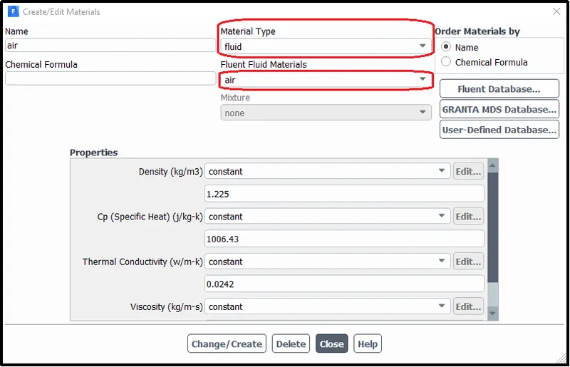
Air

For the fluid or coolant air used in the fluid domain.

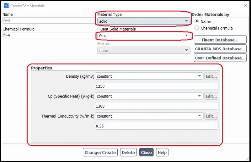
FR-4

FR-4 is a glass-reinforced epoxy resin laminate that stands for “Flame retardant”. it has a high working temperature, good heat resistance, good moisture resistance, good hole metallization performance. Therefore it is preferred to build PCB.

In this project, the base plate is considered as a circuit board so FR-4 material was used for it.

FR-4 material is not present in fluent therefore it was created, for this simulation, using user define material by changing the name and properties of the existing material.

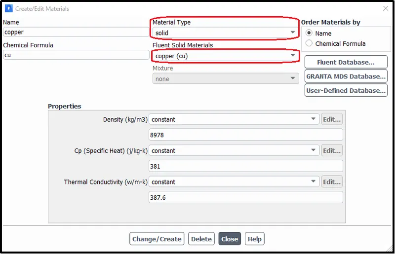
Copper

Copper is a good conductor of heat therefore it was added to assign it to fins.

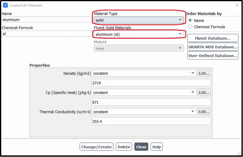
Aluminum

Aluminum is by default added by fluent so it kept as it is and used to assign for other remaining components.

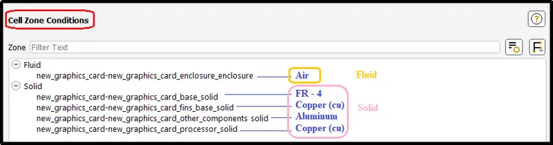
In cell zone condition material was assigned to their respective component as per portray in below picture.

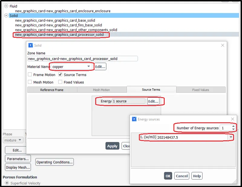
The Graphics card processor chip is the main heat source, hence, activate the source setting in fluent. Then, here, we have to define how much energy is releasing from the processor.

For this case, R350 GPU was considered which assumed to be running at 400Mhz on a 0.15micron process at 1.75v which is 51.75W output (Reference 2)

Under the full load conditions, GPU run with the efficiency between 66% to 75% rest of energy got waste in the form of heat which is 12.9375W 25% of total energy.

Now we need it in the form of per volume ( volume of the processor)

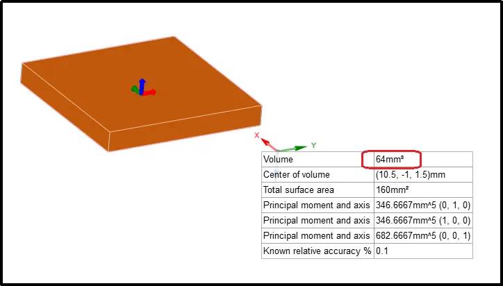
`En ergy = 12.9375/(64e-9)`

`En ergy = 202148437.5`w/`m^3`

Therefore above energy value is considered as the heat source value.

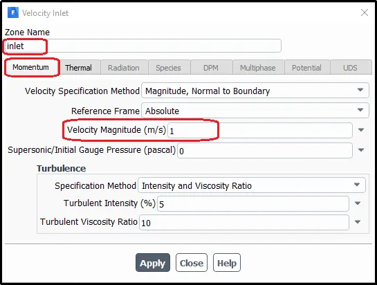
Inlet velocity was taken as 1m/s

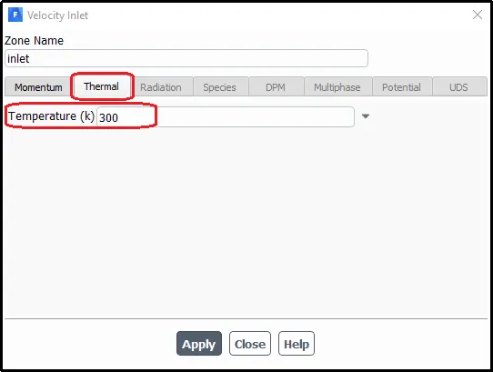
Normal inlet air temperature is considered as 300K.

After setting up the setup solution was run for 100 iterations

Solution convergence

Residual plot:-

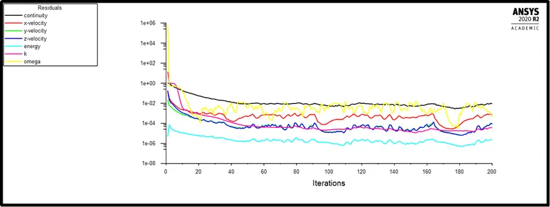
The residual chart exhibits that all the entities giving fluctuating results in the same range as the results getting calculated with the number of iterations. Therefore we can stop at the 200^th iteration and considered it as a converged result.

The average temperature of the solid faces

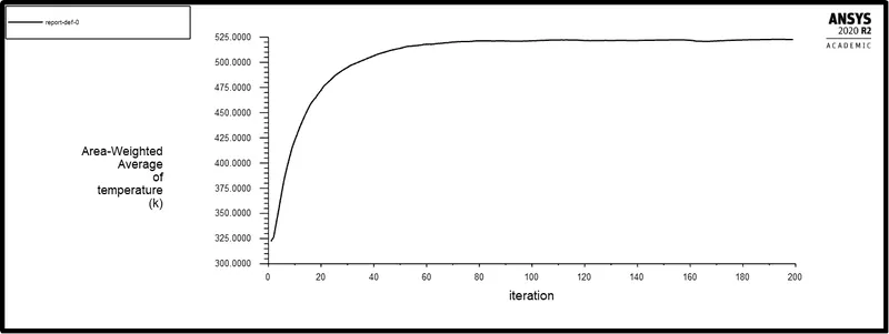
Another way to confirm that results are converged or not is by observing the Average temperature of the solid. As the table flow after a particular time, the temperature of solids also maintains its temperature in a very minimum constant range which shows the final solution is achieved.

Average Y-plus value:-

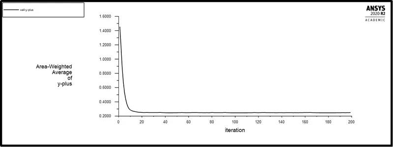
The average Y plus value:- 0.25054672

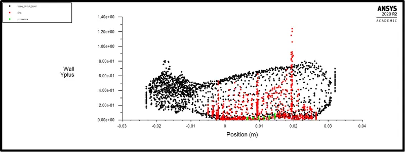
Here maximum Y+ value is showing somewhere around 1.2 to 1.3 which is already low but in this study, our geometry size is also small. Therefore for final geometry y+ maintained below 0.5.

The Average Heat Transfer Coefficient:-

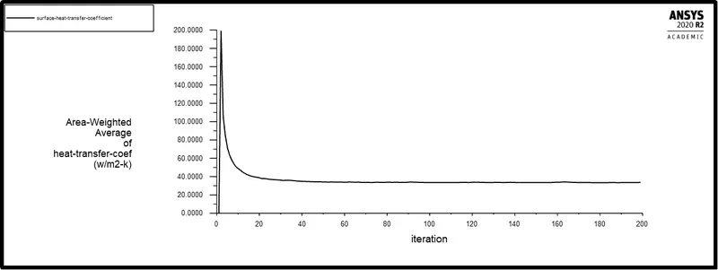
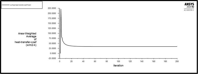
The heat transfer coefficient achieved by coarse mesh for 1m/s velocity is 33.634619W/m²-K.

Meshing:-

Final mesh:-

For first layer thickness 0.33334, we are getting 1.3 as a maximum Y+ Value by coarse baseline mesh. So to get Y+ = 0.5 we should use the first layer thickness as 0.1282.

So total thickness can be calculated as

First cell height in mm

dY = 0.1282mm

Number of layers

n = 4

Growth rate

Gr = 1.2

Therefore, total thickness we got is

`Tt = dY xx (Gr^(n-1))`

`Tt = 0.2215 ~ 0.2`

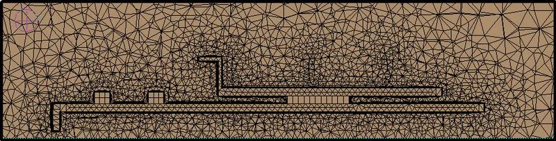
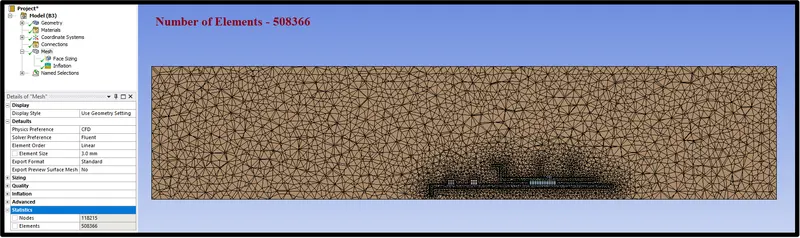
Here element size for the solid surface set for 0.72mm to get fine mesh near the wall surface.

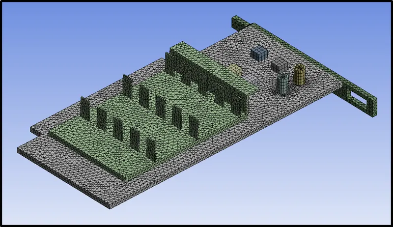
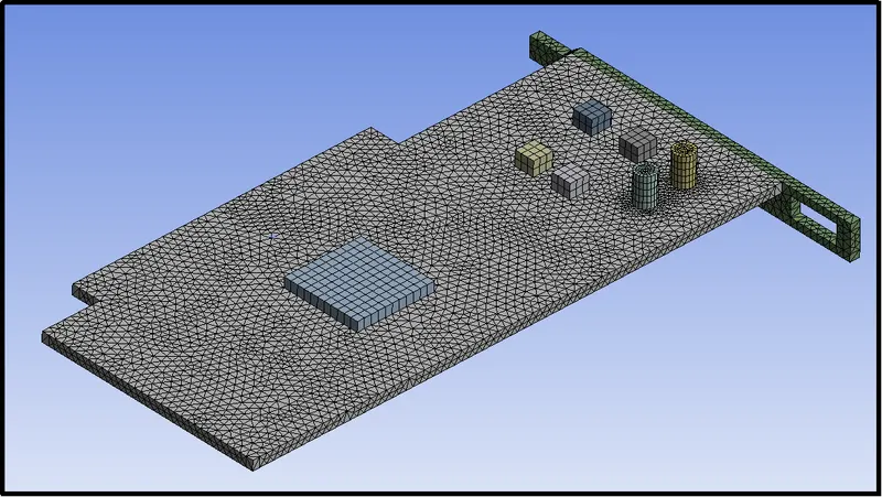
Element size for the fluid domain was set for 3mm by which the number of element achieved is 508366 which is less than 512000(cell limit of Ansys Student version)

Fluent setup

Fluent setup kept same as setup of a baseline mesh and solution is ran for the same number of iterations which is 200.

Convergence of solution

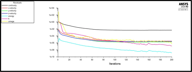
Residuals:-

in the residual chart, every entity's values coming in a constant range after somewhere around 160 iterations therefore we can say that evaluating the solution till the 200 iterations is enough.

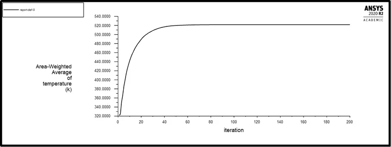
The Average Temperature of solid walls:-

Another way to declare the convergence of the solution is to observe the average wall temperature for the constant inlet flow. The average heat transfer is showing is 521.6761 ^oK

Average Y-plus value:-

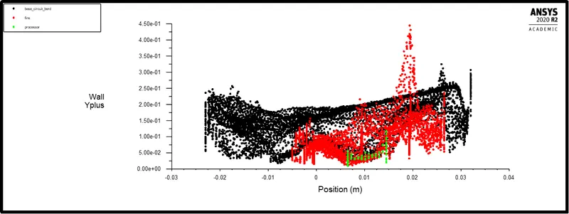
The Average Y+ values we got from this case is 0.25054672

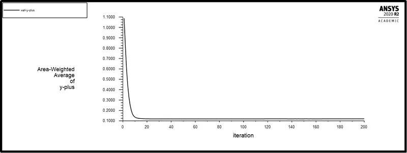
Here the maximum Y+ value is less than 0.45 which is near our Y+ analytical calculation.

The Average Heat Transfer Coefficient:-

The average Surface Heat transfer showing for this problem is 34.259515 W/m²-k

Mesh Independency check:-

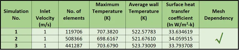
In the first three simulations, we ran a solution for 1m/s velocity to check the mesh independence. And with each case we got results in a very close range, hence, the mesh is dependable. Therefore, for further simulations, for velocity 3m/s and 5m/s, the same duplicate setup was used.

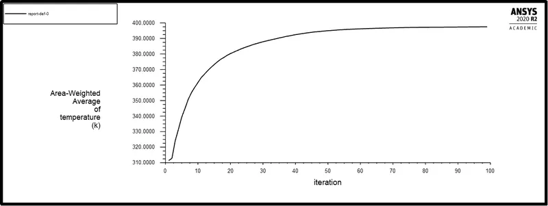
Results from the fourth simulation with 3m/s velocity:

The Average Heat Transfer Coefficient:-

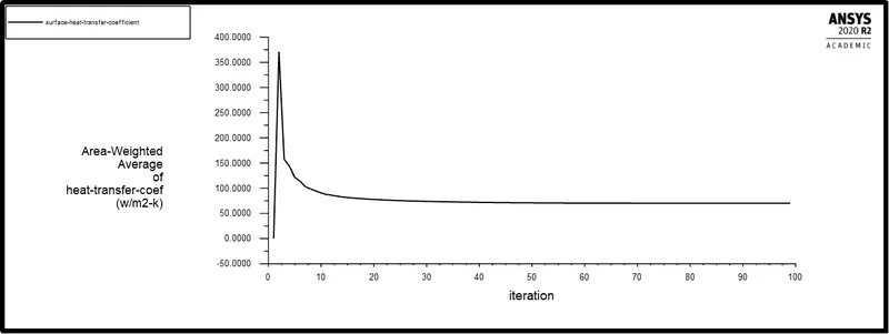
The average heat transfer coefficient for 3m/s velocity is 70.076204 w/m2-k

The Average Temperature of solid walls:-

The average temperature of the solid wall faces for 3m/s velocity inlet is 397.51423 ^oK

Results from the fifth simulation with 5m/s velocity:-

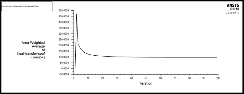
The Average Heat Transfer Coefficient:-

The average heat transfer coefficient for 5m/s velocity is 70.076204 w/m2-k

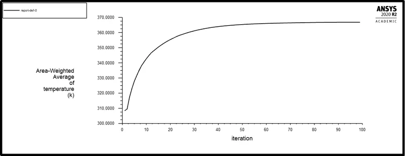
The Average Temperature of solid walls:-

The average temperature of the solid surfaces for a 5m/s velocity inlet is 366.79489 ^oK

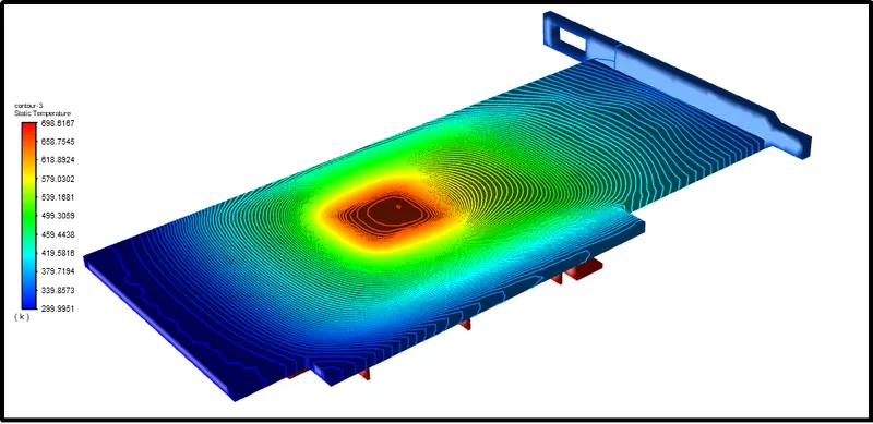
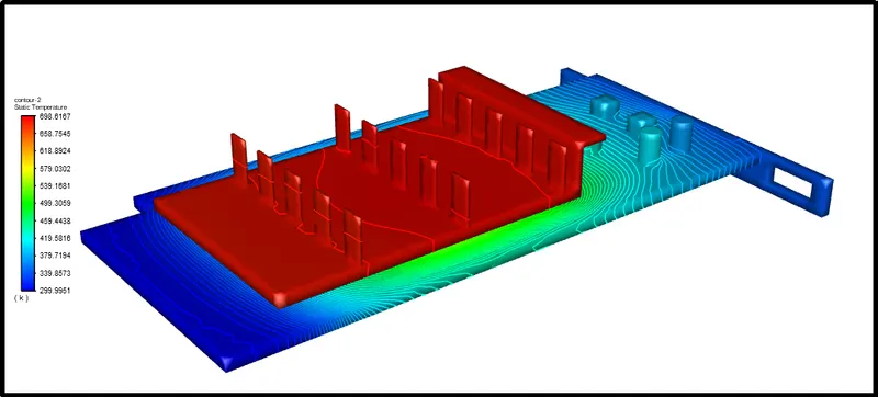
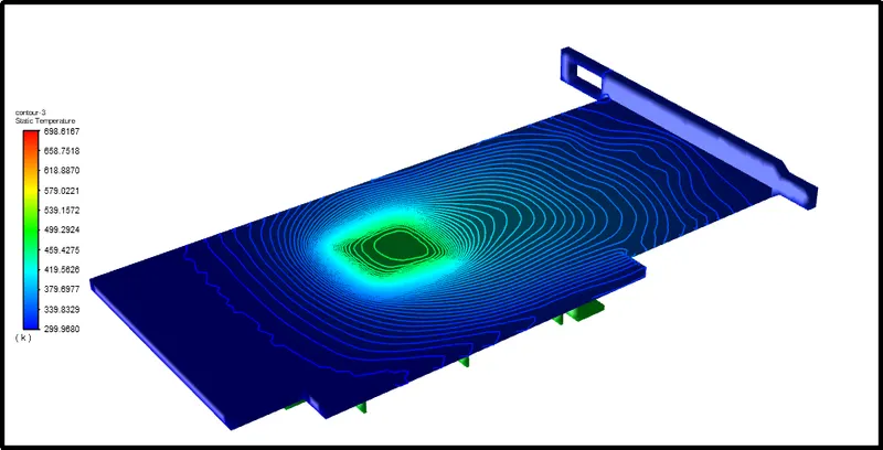
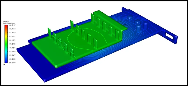
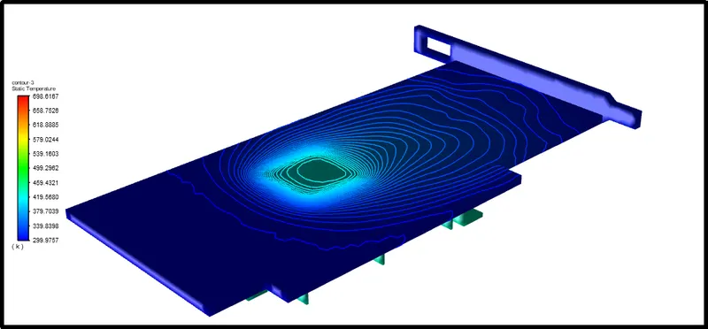
Temperature Plots (temperature Range:- 299.9951 ^oK - 698.6167 ^oK)

For 1m/s velocity

The backside of the circuit

Upperside of the fin base and fins

For 3m/s velocity

The backside of the circuit

Upperside of the fin base and fins

For 5m/s velocity

The backside of the circuit

Upperside of the fin base and fins

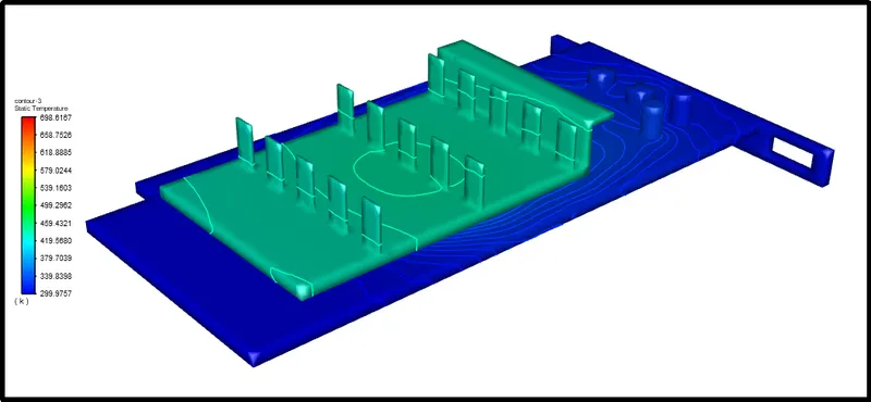
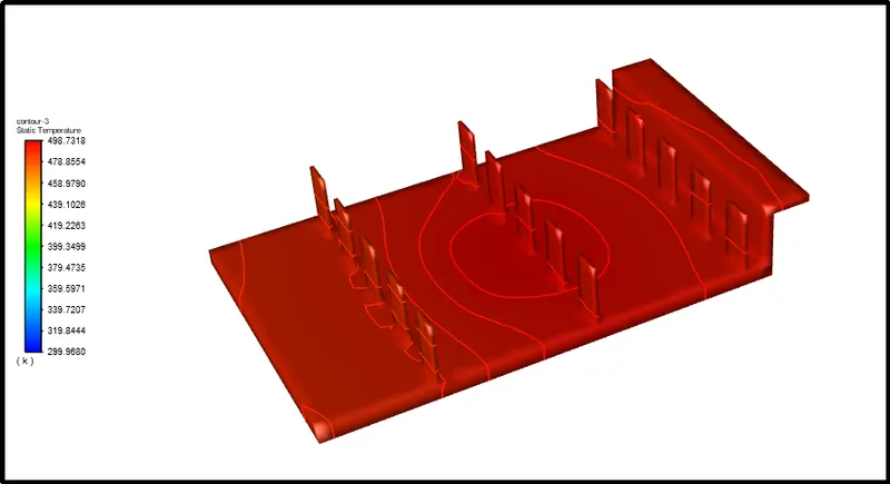
The above pictures exhibit the temperature contours on a surface of components for the velocity 1m/s, 3m/s, and 5m/s, for temperature range (299.9951-698.6167) respectively. Here we can clearly observe the heat transfer rate increases as the velocity of the inlet flow increasing.

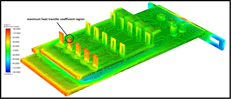
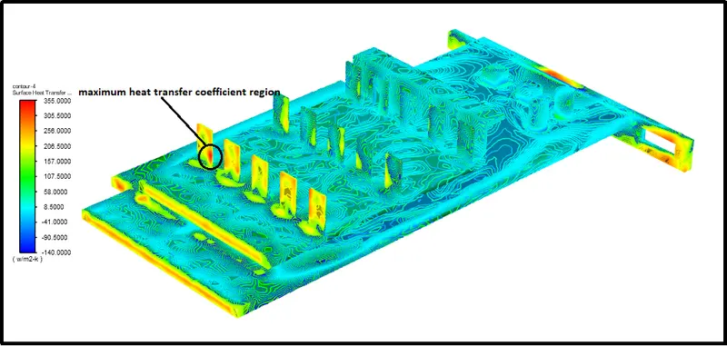
Maximum Heat Transfer Coefficient area

For 1m/s velocity

The heat transfer coefficient is very high at the boundary surface of the first row of fines where the pressure is very low and velocity is increasing.

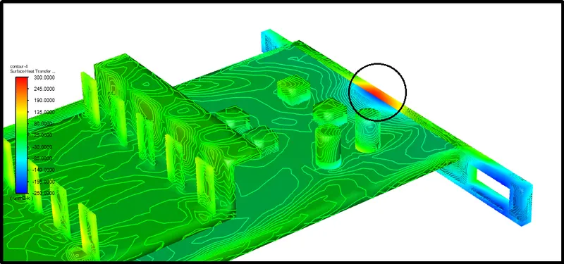
For 3m/s velocity

For the 3m/s the heat transfer coefficient is showing high on the last component attached to the base plate because the velocity there is high. But for the heat dissipation, we need the high HTC near the fin and base plate area. Therefore those components can be ignored and the fin processor and base plate only considered to get proper heat transfer coefficient.

Now we are getting the maximum heat transfer near the boundary of the fins on the first row.

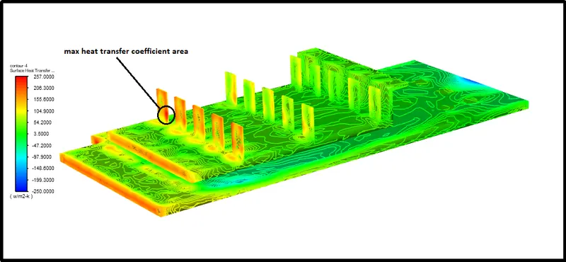
For 5m/s velocity

The same thing is happening for the input velocity 5m/s we got the higher heat transfer coefficient near the boundary of the fins in the first row because the velocity is increasing near the boundary of the fins.

Final Observations:-

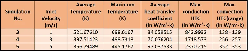
From observation from the above table, we can notice that the heat transfer coefficient is rising as the velocity is increasing which is directly related to the greater heat transfer rate. in this model, we want better cooling of graphics card which one can achieve with larger inlet velocity (5m/s).

Potential hotspots on the model

Only potential hotspots can observe here is on the circuit board, as the FR-4 is not a good conductor of heat but it can withstand a high amount of heat therefore is used to manufacture PCBs.

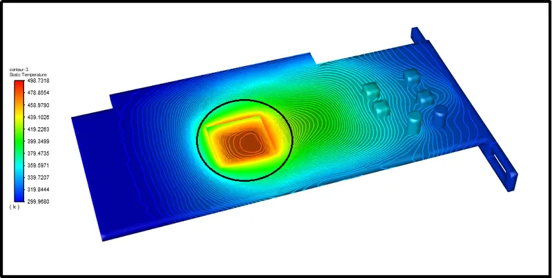
Other than that, copper is a good conductor of heat and hence, it is distributing the heat properly to the overall surface area and providing a better heat dissipation effect with a higher heat transfer rate.

Conclusion:-

• Higher velocity in a particular region means a higher Reynolds number. That’s why the heat transfer coefficient in that area is highest, which means the maximum amount of heat transfer is taking place from fluid to the solid in that region. This also results in a higher temperature of solid in that location.
• Heat transfer coefficient is a function of properties of the fluid at film temperature, temperature difference, temperature coefficient, buoyance force et, hence, mesh resolution near walls usually has the biggest impact on numerical results.
• For the turbulent models, we have to take care of the assumptions and the boundary conditions you put in the program. The mesh is a very important parameter to get nice results so we have to refine it in the important place of our drawing.
• Some factors should be considered which the most significant is the turbulent boundary layer. If we are using any kind of low Reynolds turbulence model considering enhanced wall treatment (as your K-w SST model), so we need to make sure that we stay in the laminar sub-layer region where velocity profiles are assumed to be laminar and viscous stress dominates the wall shear which means
• Mesh/ grid dependency test is very important to get confidence over results.

References:-

[1] PCB FR4 - https://www.proto-electronics.com/blog/pcb-fr4-guide-printed-circuits

[2] The heat output of GPU - https://www.overclockers.com/forums/showthread.php/279469-Calculating-the-heat-output-of-a-GPU