Week-6 Calculate the Stretch Ratio by comparing the ELFORM (-2,-1,1,2) with Ogden_Material Model.

STRETCH RATIO COMPARISON BY DIFFERENT ELFORM:

OBJECTIVE:

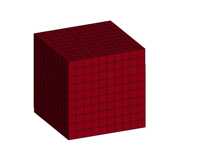
The objective of this project is to create a cube of dimension 10x10x10 (mm) modeled using a solid element and Ogden Rubber, a hyperelastic material. Upon this model, a tensile force is applied as a loading condition while the other end is constrained in space and hence to determine the stretch ratio when the solid is modeled using different element formulations like 1,2,-1,-2.

KEYWORD SETUP:

1. MODEL GENERATION

The model can be created within LS-PrePost as follows,

Mesh -> ShapeM -> BoxSolid -> (define region) -> (define mesh elements) -> Name=cube

The above commands will let users create a solid block whose nodal positions in space can be defined and the mesh elements that need to be generated along with all three x,y, and z-axis can also be specified.

2. *PART - *SECTION & *MA

All units are in gm/mm/ms

The created part is modeled using the MAT_77_O-OGDEN-RUBBER, which can also be termed as a HyperElastic-Ogden-Vulcanized Rubber. The section of the part model is a solid section that can be assigned using the keyword *SECTION_SOLID. This part is modeled using 4 different cases each saved in a separate keyword file hence can be run individually.

The four different cases that are modeled are modeled using SECTION_SOLID with 4 different element formulations, namely:

ELFORM 1 - constant stress solid element

ELFORM 2 - fully integrated S/R solid

ELFORM -1 - fully integrated S/R solid intended for elements with poor aspect ratio, efficient formulation.

ELFORM -2 - fully integrated S/R solid intended for elements with poor aspect ratio, accurate formulation.

• Solid formulation 2 most often employs a B-bar method and thereby assumes that pressure is constant throughout the element to avoid pressure locking during nearly incompressible flow.
• Solid formulations -1 and -2 employ an assumed strain approach to avoid the shear locking behavior seen in formulation 2 elements that have poor aspect ratios.
• Formulation -1 is a more computationally efficient implementation of formulation -2.
• Formulation -1 has a side effect that resistance to a particular deformation mode, similar to an hourglass mode, is weakened. This side effect is
  not truly hourglassing behavior, so there is no hourglass energy and the behavior is not affected by hourglass parameters.

3. *BOUNDARY

The required boundary conditions are applied using this keyword.

BOUNDARY_SPC_SET:

This keyword is used to constrain a given set of selected nodes on the part along/about x, y, and z-axis. In our case, the nodes present at the left end of the part is constrained in all DOFs using this keyword.

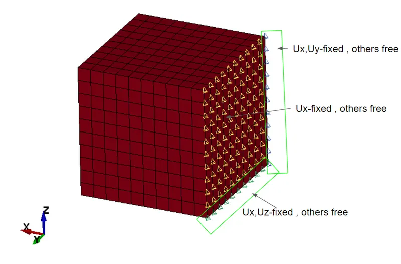
BOUNDARY_PRESCRIBED_MOTION_SET:

This keyword is used to apply a loading condition to the node sets of the part model. The required node sets over which the loading is applied can be specified using SET_NODES from CreEnt.

In our case, a Prescribed motion is applied in terms of displacement and other parameters as shown below,

stretch ratio `lamda=1+epsilon_e` where `epsilon_e` is engineering strain

since we consider stretch ratio as 5

then

`5 =1+(deltal)/10`

`deltal=40 mm`

we are defining a stretch distance of 50 mm(>40 mm) as input load.

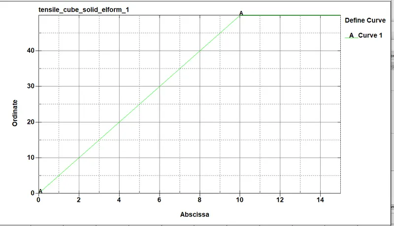
The LCID is used to define the load Curve, which controls the rate at which the displacement is to be applied based on time.

3. DATABASE

This keyword is used to specify the desired output results that need to be extracted from the analysis. The most important keyword is *DATABASE_BINARYD3PLOT. This keyword is used to write the simulation results onto a file that can be used to view the animation of the simulation using LS-PrePost.

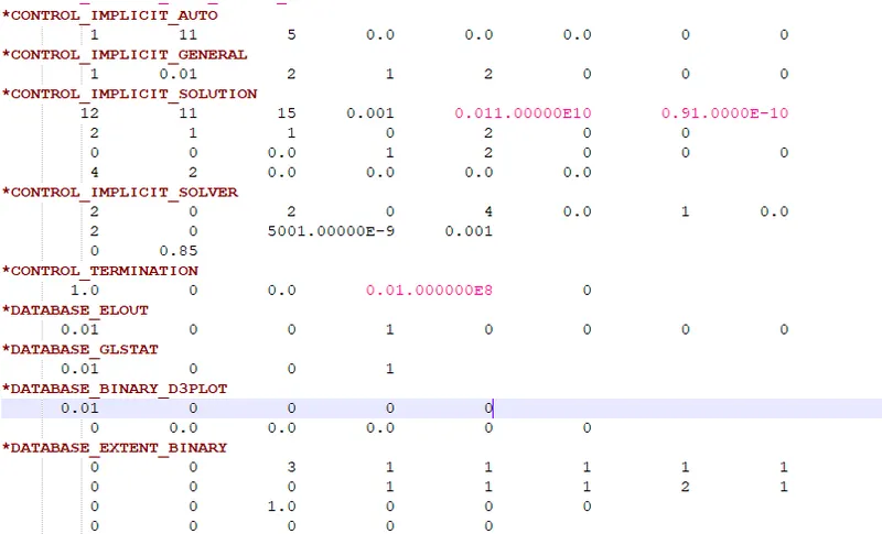
The necessary parameter for this keyword is the time interval (DT), which specifies the frequency at which the animation file needs to be written. In our case, we specify DT=0.01ms.

4. CONTROL

TERMINATION:

This keyword is used to define the termination or end time of the simulation which will be 1.0 ms

IMPLICIT_GENERAL:

For this simulation, the Implicit method will be used rather than the default explicit method. The reason being our analysis is a quasi-static analysis since it involves large deformation but under the static condition and the other reason being our simulation is time-independent however loads are given in steps.

The IMFLAG parameter is set to 1 thereby activating the implicit solver and a DT0 (initial time step) of 0.01ms is set.

NOTE: Explicit method is preferred for highly Non-Linear transient analysis which occurs within a fraction of seconds and transient meaning time-dependent.

IMPLICIT_SOLUTION:

This keyword is defined in case there occurs non-linearity in our problem. Since our problem involves large displacement, it is advisable to use this keyword since our problem is solved using implicit methods.

The NSOLVR parameter is set to 12 (Nonlinear with BFGS updates + optional arclength), which is the default Non-linear solver for most implicit methods. The matrix refinement parameters namely, ILIMIT and MAXREF can be set at a relatively low value since once running the simulation we could notice that each step is solved within two iterations. The other important parameters DCTOL (Displacement convergence tolerance) is set to 0.001.

IMPLICIT_SOLVER:

Same as specifying a Non-linear solver, this keyword lets us choose a specific Linear solver that will be suitable for our analysis. In this case, we will set LSOLVR=4 as a "SMPparallelmulti-frontal sparse solver".In this case, we will set an LSOLVR of 4 which is an SMP parallel multifrontal sparse solver.

--------------------------------------------------------------------------------------------------------------------------------------------------------

POST_PROCESSING:

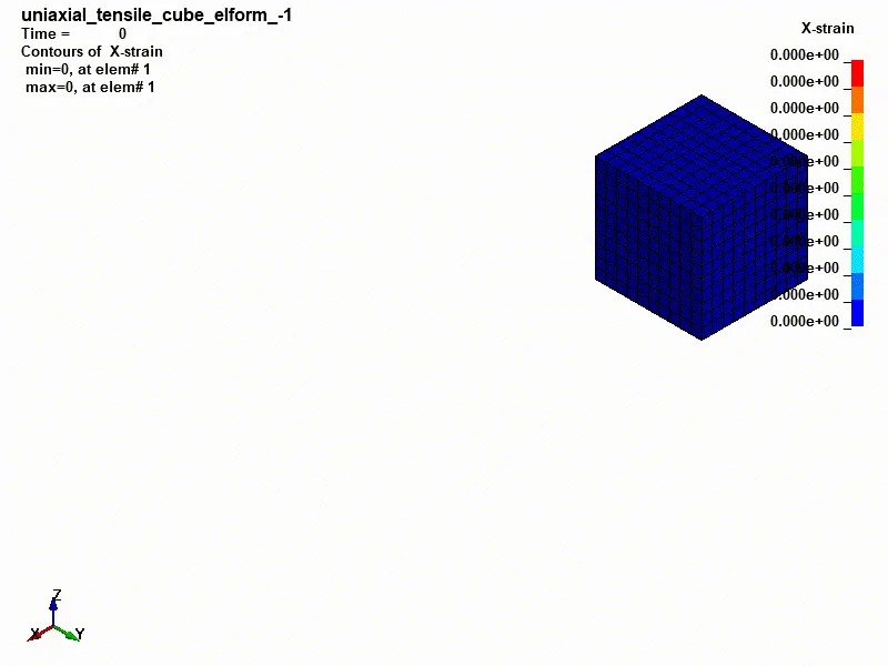
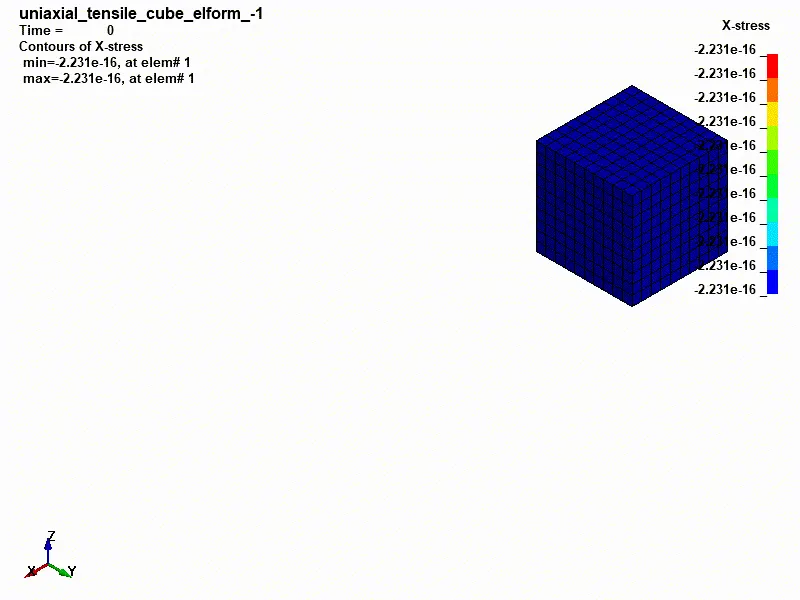
The above analysis defined and modified in four different keyword files are computed using the LS-DYNA solver and the following results have been extracted,

X-strain:

X-stress:

The process of attaining the results from post-processing and the end result in the Stretch ratio as detailed below,

• Select an element from the part and plot its stress and strain data individually using the History tab in post-processing.
• Save this data onto a .csv file thereby exporting the potential stress and strain data onto a valid format.
• This data in .csv format can be viewed and modified in an excel sheet.
• Using the XY Plot the written .csv file can be imported to plot the Strain in the x-axis and the Stress data in the y-axis. (as shown in the figures)
• To calculate the Stretch:

--------------------------------------------------------------------------------------------------------------------------------------------------------

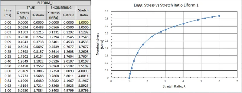
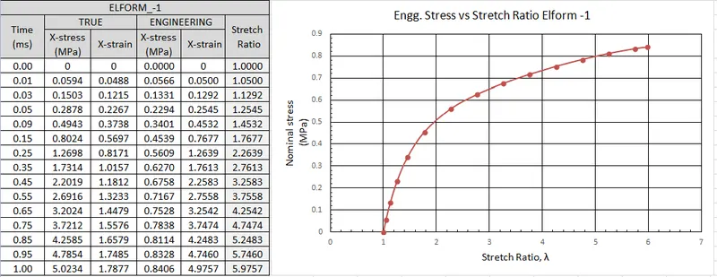
Calculation of stretch ratio:

True strain = ln(1 + engineering strain)

True stress = (engineering stress) * exp(true strain) = (engineering stress) * (1 + engineering strain)

stretch ratio = 1+ engineering strain

Elform=1 constant stress solid element

Elform=-1 fully integrated S/R solid intended for elements with poor aspect ratio, efficient formulation.

Elform=2 fully integrated S/R solid

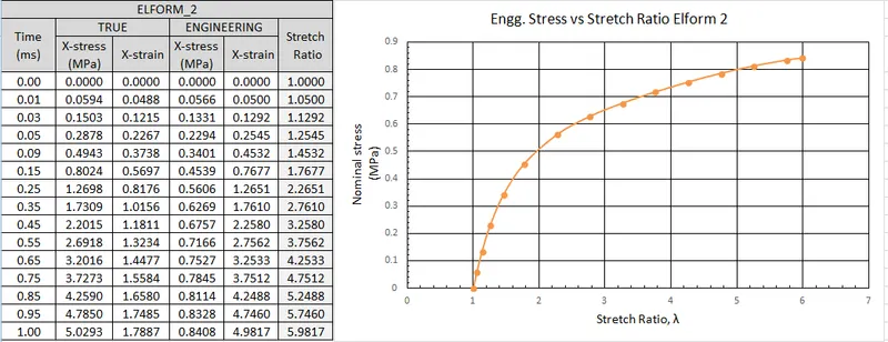
Elform=-2 fully integrated S/R solid intended for elements with poor aspect ratio, efficient formulation.

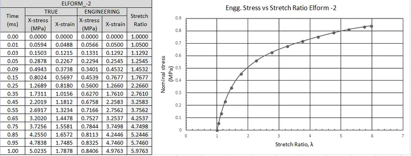
Comparison of analysis result with given data:

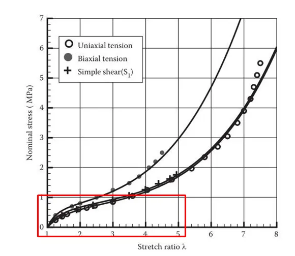
given data:

results from the analysis:

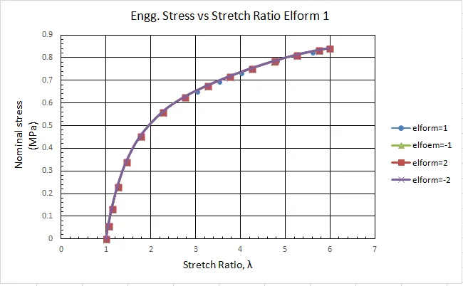
it can be seen that results for elform 1,-1,2,-2 are all same. but if the stretch ratio is increased solution for elform 1,2 will not converge due to poor element quality(aspect ratio) so elform -1 or -2 has to be used.

And results slightly vary from the given data because of,

• assumptions in material modeling for FEA where the stress-strain curve is defined as three linear curves.
• element size (mesh convergence study has to be done to verify the results.
• Assumption sin element formulations.
• Near perfect boundary conditions which is not possible in real experiments

CONCLUSION:

From the above-obtained results, the results of different solid elements modeled using different element formulations is negligible.

The material that is used to model the part also tells us a lot about the deformations that occurred. Since the MAT_077 is a hyperelastic material we can notice a huge deformation after the yield point while this would not be the case in other materials that possess high stiffness.

Results vary slightly from experimental data because we have modeled the non-linear region of the material curve as three linear regions

the change in stress is not linear to the change in strain or stretch but the relation between them is parabolic in nature. This means that during the initial time steps the resistance offered by the solid object is high causing a small stretch ratio. However, as the displacement acting upon the part gradually increases based on the specified load curve we can notice an exponential increase in stretch reason being very small resistance is being offered by the body as it is well beyond its yield point.