Week-6 Calculate the Stretch Ratio by comparing the ELFORM (-2,-1,1,2) with Ogden_Material Model.

WEEK 6 Calculate the stretch ratio by comparing the ELFORM (-2,-1,1,2 ) with Ogden_Material Model.

Aim-

Given is an Ogden material card which is hyperelastic (rubber). Create a 10x10x10mm solid mesh and run a pure tensile run on it with a stretch ratio of 5. Compare different element formulations of solids 1,-1,2,-2 and plot engineering stress vs stretch values

Explanation-

Since this simulation is happening at a really slow pace (quasi-static) the inertial effects can be neglected we can consider implicit for the analysis.

Since this is a hyperelastic material even though we are running it in implicit, we need steps and iterations to achieve the equilibrium.

Element formulations used are 1,-1,2,-2 for solids.

ELFORM 1 - under integrated constant stress; needs hourglass stabilization; efficient and accurate

ELFORM 2 - Reduced integrated; no hourglass stabilization needed; slower than ELFORM 1; shear locking can occur

ELFORM(-1 )- similar to ELFORM 2, but shear locking is accounted for; efficient formulation (CPU time)

ELFORM (-2) - Similiar to -1, more accurate, more computational cost.

Procedure-

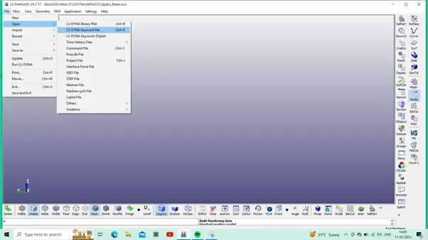
• We have to open the given LS-Dyna keyword (.k file) file in LS-PrePost, using the option File>Open>LS-Dyna Keyword File as shown in the below snap.

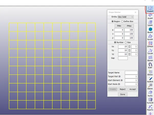
• Now we will open Ogden.k file and create the cube of size 10mm X 10mm X 10mm.

• First we will start with section card, to create section card from keyword>>all>>section>>solid>>here we will input id, elform type as shown below.

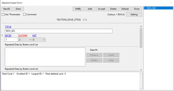
• As per given cases we have to change ELFORM as 1, -1 & 2,-2, accordingly as shown in above snap or we can do it from .k file after saving it.
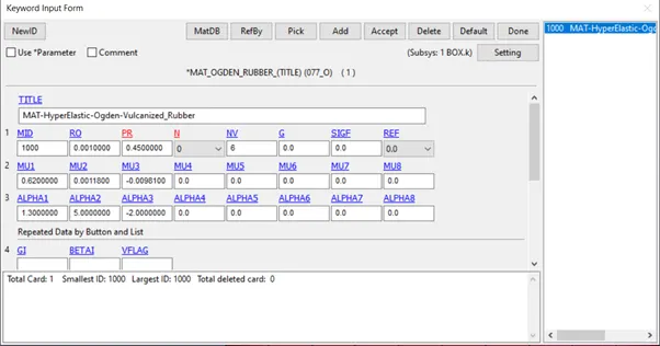
• Now we will check the MAT card given to us.

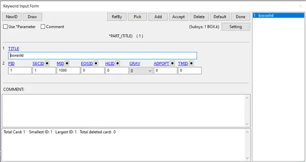
Finally we have to assign the section and material to the part.

• Here we will fix the Bottom of the Cube and give the motion to the set of nodes on the Upper face.
• To fix the Bottom face, we will use different set of nodes and using single point constraint boundary, we can allow or constraint the nodes with different degrees of freedom.
• We have use different node set so that we can mimic actual tension representation of the rubber box
• First we create node set along y axis having , are free to move along y axis
• Second set have node set along x axis ,and are free to move along x axis
• Third set will include all remaining node from that face , which are free to move in XY plane

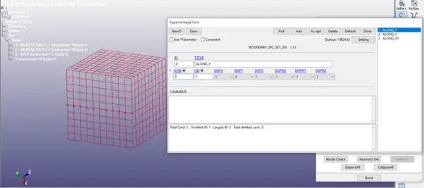
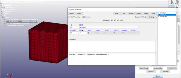
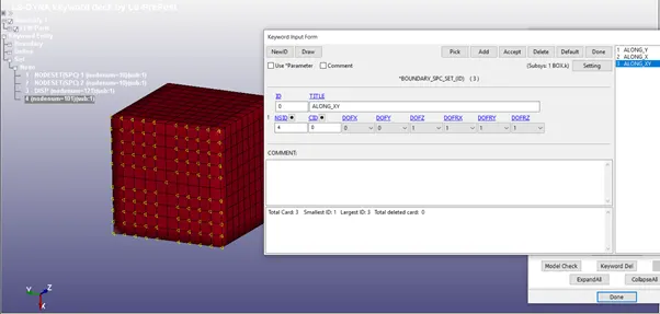
• As shown in above image, constraints are given for the different set of nodes in a way that cube can shrink in X and Y direction upon tension in Z-Direction and also stick to its position.
• Thus , this boundary condition can be relatable to the real-time boundary condition.
• To apply the tensile load in Z-Direction to the cube, we have to give the motion to the set of node on the upper face of the cube.

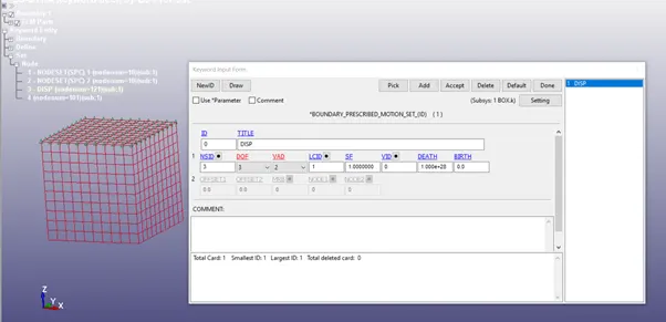
• As shown in above image, we have given DOF = 3 , to allow translation in Z-Direction translation
• VAD = 2 is given for Displacement.
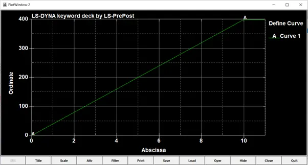
• We will define curve for displacement is given below, displacement is linearly applied at constat rate

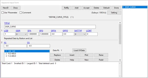
We know that Stretch = 1 + Engg strain

=> 5 = 1 + (change in length / 10)

=> Displacement(change in length) = 40mm

LS-Dyna employs both implicit and explicit methods to solve Static, Quasi-Static and Dynamic problems.

• These problems can differ in Time Increment approach.
• In implicit each Time increment has to converge, but we can set quite long time increments.
• In explicit, convergence for each time step is not needed.
• In implicit method, at each time increment, global equilibrium is established, due to iterative method.
• Implicit method is used for accuracy and can be applied for long duration problems.
• Also implicit methods are used when the deformation is not so large or the deformation is happening in a gradual manner.
• Here, we are stretch the cube up to 40 mm, is large deformation, but for the hyper elastic materials, this deformation can be small.
• So, implicit scheme is best for this type of analysis.

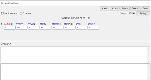
• Since this is the nonlinear implicit analysis, we need to create some implicit cards to activate implicit method like implicit auto, implicit general etc as given below:

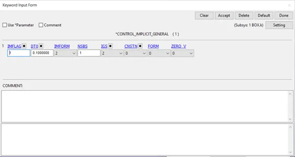
• In *CONTOL_IMPLICIT_GENERAL, IMFLAG =1 is given to activate the implicit analysis method and initial Time step value is given as 0.1.
• In *CONTROL_IMPLICIT_AUTO, values of DTMIN and DTMAX are not defined, so that the solver can change the time step size as needed automatically.
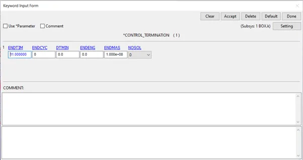
• In CONTROL_TERINATION, ENDTIM is set to 10. Here termination does not represent the time but gives the value at which step the analysis will end.
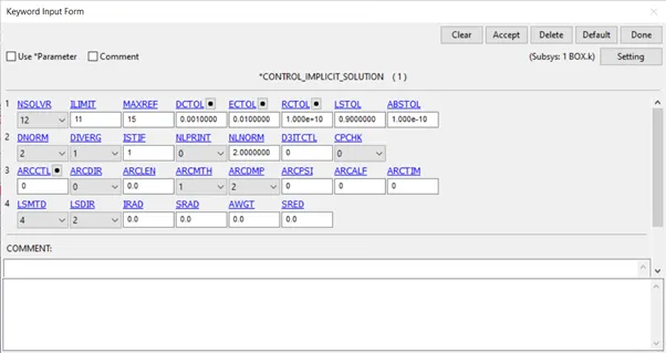
• The nonlinear solver parameters are set on *CONTROL_IMPLICIT_SOLUTION where the solver type is specified as NSOLVR = nonlinear or linear implicit analysis option

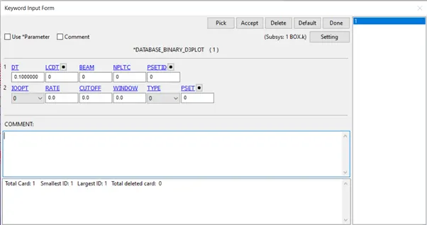
Now we will provide database output parameters to get the required results as d3plot and ascii plot files

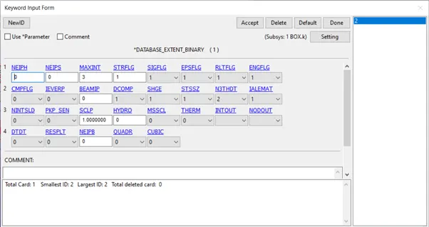
• Now we have to check the model from model checker.

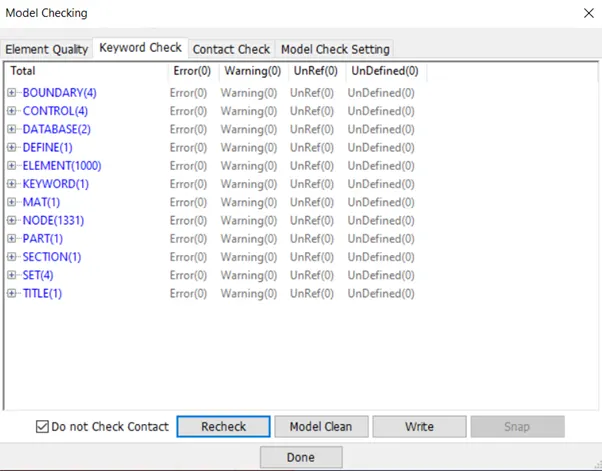
Since there is no error we can proceed further to save and run the keyword file .

Once simulation is done we can move to post processing

Results & Plots:

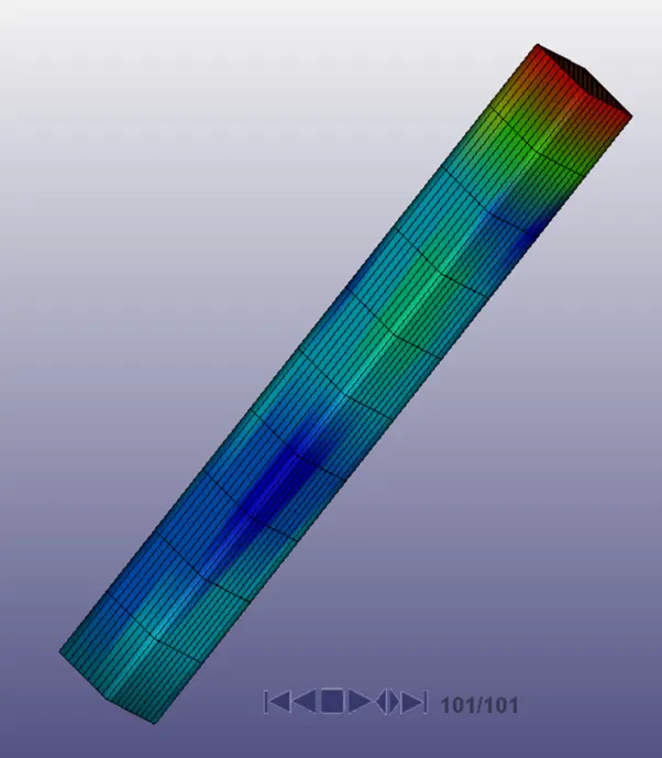
Stresses in Z

Elform 1

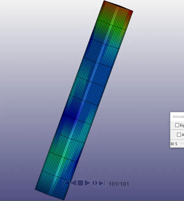
Elform 2

Elform -1

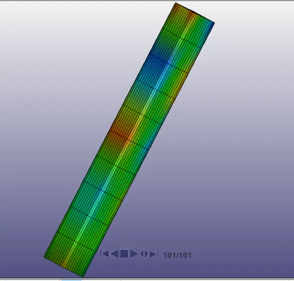
Elform -2

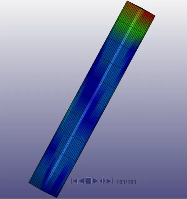
We can see the stress results for different element formulations.

Maximum stress we obtain is 4 Mpa along the Z-direction. As the tension is applied in Z-direction.

We can observe the same value of maximum stress for all cases, but the distribution of stress is different in all cases.

Similarly the maximum strain in Z direction is 1.6028, which is same for all cases.

Calculation of Nominal Stress & Stretch Ratio:

Now we will see the calculation of the Nominal Stress and Stretch Ratio for all cases.

• After getting the values of True strain and True stress from the plots, we can use the XY data and export it as “CSV” file and open it in EXCEL.
• Here all the data of True Stress and rue Strain are collected for all cases using an element results from the middle of the cube, which is Element 500.
• So all the results will be regarding Element ID: 500
• Here Stress results for Element 500 will be from Z-Stress
• Strain results for Element 500 will be from Lower Ipt Z-Strain.

Stretch Ratio:

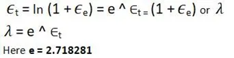
• Here we can get the Stretch ratio from the True strain.
• To get the Stretch ratio, we can use formula as given below:

Nominal Stress:

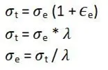
• Here Nominal stress is the Engineering stress in Z-Direction.
• To get the Nominal Stress, we can use the formula as given below:

Calculations and the result data for all cases are same as given below:

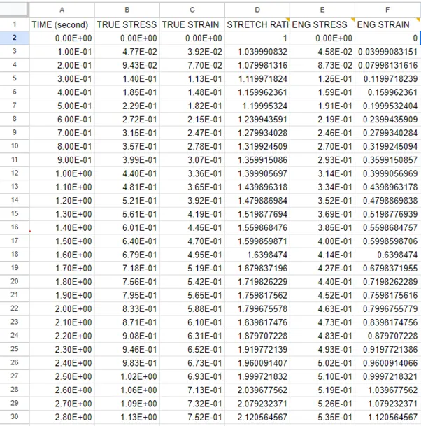
• From these values of stress and stretch ratios, we can create the graph of Nominal Stress Vs Stretch ratio for all element formulations.

Plots:

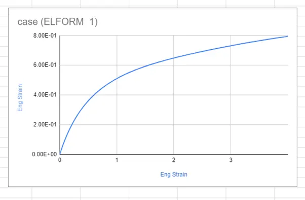
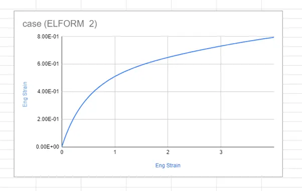
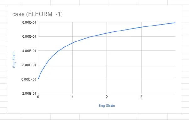
Plots of Nominal Stress Vs Stretch Ratio for Element formulation 1, 2,-1, and -2 as per case will be as given below:

Comparison:

• Plots obtained from the simulation results, we can observe the Stress and Strain results are same for different solid element formulations.
• We can observe same stretch ratio for all different element formulations.
• But we can see the distribution of stress over the length of the cube is in different manner while stretching. This is due to different behavior of element formulations.

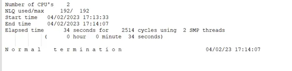
Elform 1

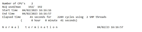
Elform 2

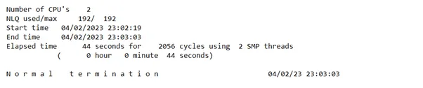
Elform -1

Elform -2

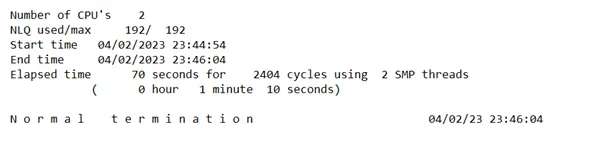
• From above Snaps, we can observe different cycles and computational time for different element formulation.
• We can see that in case of element formulation -2, it is taking highest time for computation.

Conclusion:

Since this is the uniaxial tensile test, we are getting similar results for different element formulations.

Also the deformation we have given to the cube was not so large for this type of hyper elastic material, so the difference cannot be observed.

Since the element formulation (1) is constant stress solid element, which default, cosserat point element is invoked, which is good to propose the strain energy function.

Element formulation (2) is selective reduced integrated solid element, which give constant pressure throughout the element to avoid pressure locking, but type (1) is more accurate the type (2) for implicit problems.

Element formulations type (-1) and (-2) are fully integrated elements intended for elements with poor aspect ratios. Among which type (-1) is more efficient and type (-2) is more accurate formulation.

Since Element formulation (-1) has some side effects related to some particular deformation modes , we can conclude that Element formulation (-2) is more accurate and mostly preferred for the solid elements in Implicit problems.