Implementation of Connections on Rear Door FE model Using ANSA
Aim: To implement connections on the given model (rear door) using the NASTRAN deck on ANSA software.
Theory: Connections are required for a given model to have better results while performing NVH simulation. The door has many parts connected with each other in the form of welding, adhesive, bolting, and snap fittings of plastic parts. For simulation, these connections have to be defined before running the simulation.
The procedure of implementation of these connections in the door using the NASTRAN deck on ANSA software is as follows:
1)The model given was in ".nas" format. The model cannot be opened directly in the ANSA workbench. The model has to be loaded as shown in the image.
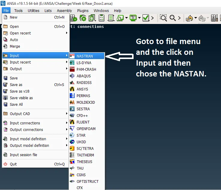
After choosing NASTRAN, goto to the directory from which the model has to be loaded.
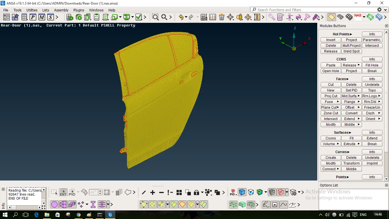
It is observed that the given is completely meshed and only connections are to be implemented.
The rigid body elements are defined using RBE2 and RBE3 connections. Most of the holes are defined using the RBE2 cluster connection.
The RBE2 are created as follows:
The RBE2 functions are found in the NASTRAN deck as in the red box in the image below and the RBE2 is the ELEMENTs toolbar (shown in the blue box). Under RBE2 there many options that are used as per the users' requirement. In the model, Many Nodes and Two Nodes options were used.
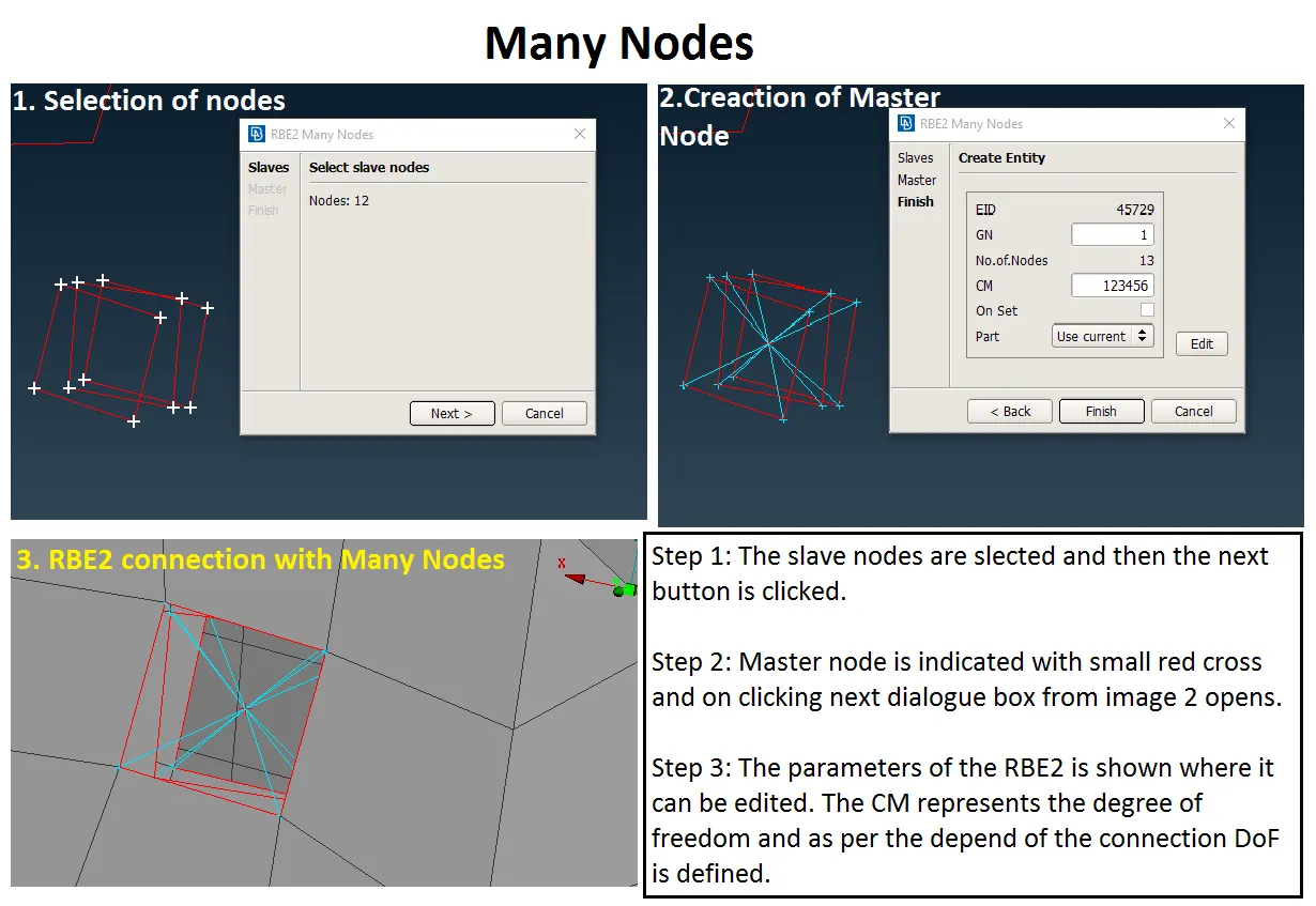
Many Nodes option:
It is used to form rigid connections on the holes. Since in the given model, the data for bolts and welds is not available. Most of the holes are represented with RBE2 Many Nodes connections.
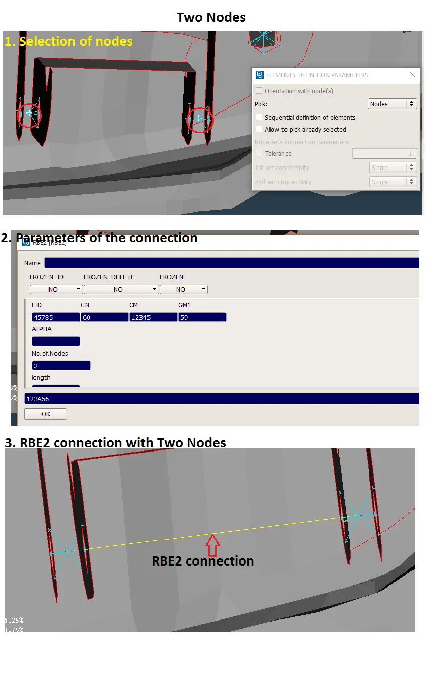
Two Nodes option:
This type of connection was used only at the door hinge. Usually, the hinge has a long stud running through it and it rotates on the z-axis. This particular connection is represented using Two Nodes with a degree of freedom limited to only the z-axis rotation thus the CM box has 12345 in it (shown in image 2). The nodes used in this are shown in the red circles in the image 1.
Representation of other rigid connection where the connection data was not available but rigidity required:
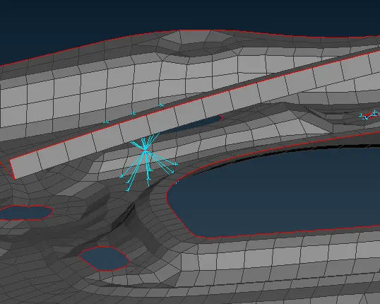
A particular pillar-like structure was bolted at one end while the other end had no defined connectivity with any other surface. The pilar did require some rigidity to be in that particular position, so an RBE2 Cluster connection with Many nodes was created (shown in the image below).
Representation of Door Handle:
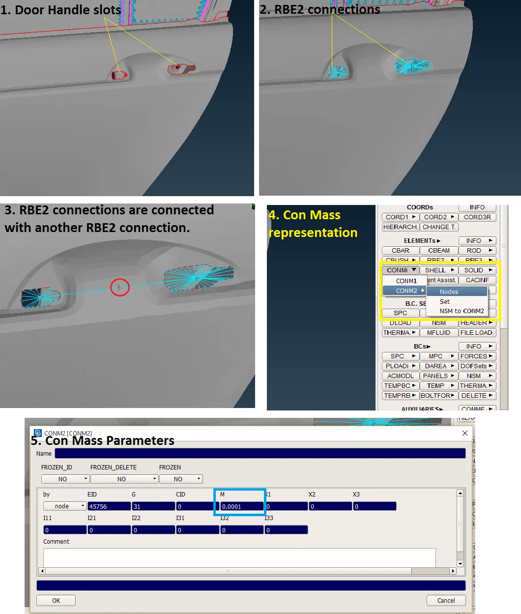
The given CAD model does not have a handle in it. The handle is represented in the form of a rigid connection to the given handle slots.
The RBE2 Many Nodes is used to create a rigid connection representing the handle (image1 & 2). The two RBE2 are connected with another RBE2 Many Nodes connection (image3).
The master node (shown in the red circle in the image3) of this newly formed rigid connection between the 2 master nodes of former RBE2 connections is given a con mass using tool CONMi in the ELEMENTs toolbar (image 4).
Since the data for the handle is not available so assumptions 100g is considered as the mass of the handle. The con mass parameters have a column M where the mass is entered. The mass units here are in tonnes so the value is entered in tonnes (image5).
Welding Connections:
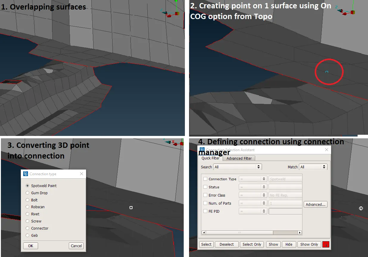
The door has many welding connections between the sheet metals but data is not given for the weld joints in the model. Assumptions of some spot weld are made and are implemented.
The spot weld is implemented at the places where the two parts overlap each other (image1). A 3D point is created on one of the surfaces using the On COG tool from Topo module (shown in Red circle in image2). The 3D point is converted into a Spotweld connection (image3). The connection defined using the connection manager (image4).
Defining the spotweld connection using the connection manager is shown below:
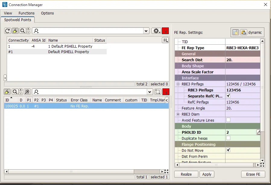
In the above image, it is seen that type of connection is shown in the tab on the LHS. The connectivity list gives the properties which are involved in a particular connection. The PIDs of both surfaces are entered in column P1 P2.
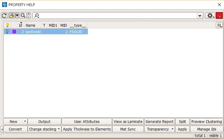
In FE Rep. Settings, the FE Rep Type is RBE3-HEXA-RBE3, the spotweld is defined using RBE3 connection. The search distance is kept at 20 and RBE3 Pinflags is given as 123456 (All DoF). The spot weld connection is a solid mesh representation so a new solid PID is created with is PID being 2 (shown in the image below). After entering all the parameters click apply and realize, the spotweld is formed.
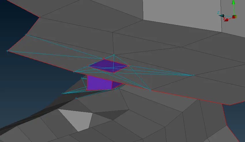
Representation of Spotweld is as follows:
Representation of Weather Strip connection to the Glass:
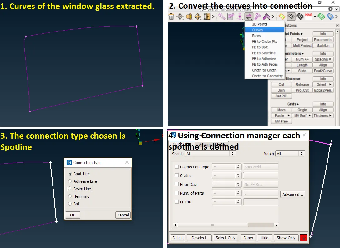
The given model doesn't have data of weatherstrip, so the curve from the glass is extracted and converted into a seamline and then the connection is defined as CBUSH-RBE3.
The curves from the FEA of glass are extracted using the Feat2Curve tool from the Mesh module. Offest one more set of curves at a distance of 10, to have a connection between glass and the other side of the door using the transform tool. Those curves are converted into spot line connection type individually. Using the connection manager each spot line is defined (shown in the image below).
Defining the connection as RBE3-CBUSH-RBE3:
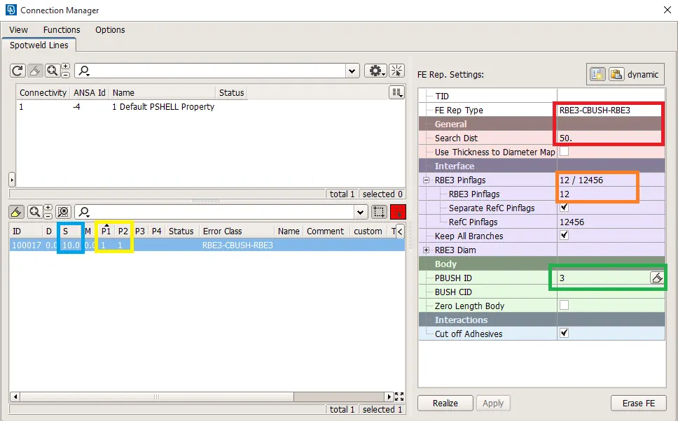
The spotlight can be chosen individually or collectively while defining the connections. The below image shows the parameters for one of the curves which have a DoF in z-axis i.e, it can move vertically in direction of window movement. The blue box indicates the space between the 2 bushes, the yellow box represents (P1 P2) the PID of the parts involved in the connections.
The FE Rep Settings are: FE Rep Type RBE3-CBUSH-RBE3 and search distance is maintained at 50 (shown in the red box). Since the window moves in a vertical direction so only 12 are included in RBE3 Pinflags (shown in the orange box). In the case of the static window in the rear door, the RBE Pinflags will include 123. The green box represents bush PID.
The bush PID is create before realizing the connection. The stiffness value (K) is entered in the parameter box as shown in the image below.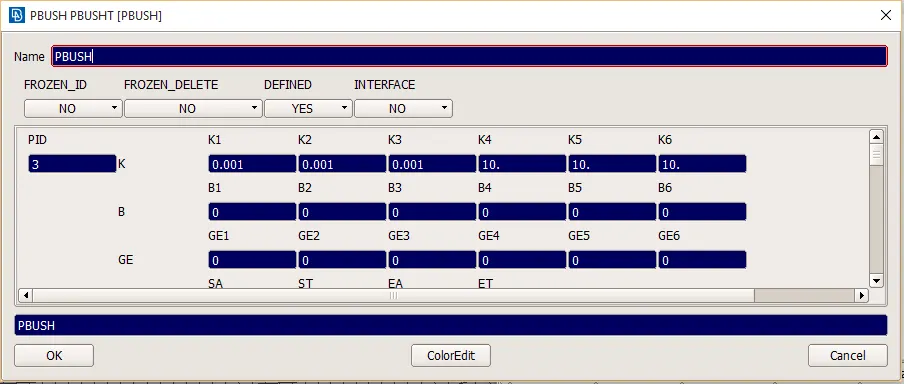
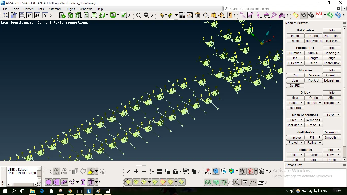
The CBUSH connection is barrel-like in yellow color it with own local axes and 2 lines connecting the glass and sheet metal surfaces (shown in the image below)
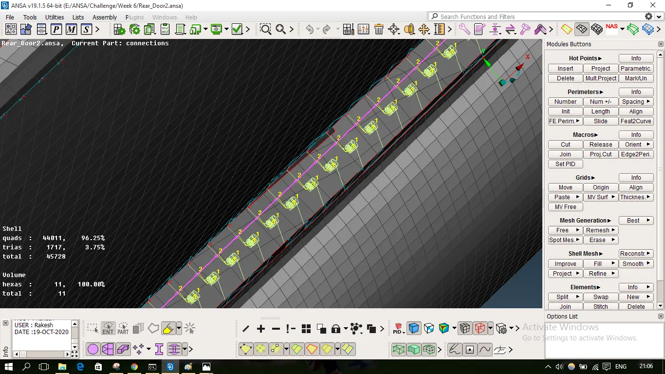
Since each bush has its own local axes and its orientation would differ from the global/vehicle axes. In order to have all the CBush orientation in accordance with the global axes, all the local axes are aligned to the global axes.
In the database, under the elements section, CBUSH data is opened on double-clicking it. It is observed that the table has the ID and name column in it representing each CBush (image 1 below).
Using hide/show columns (red box in image2) the Orient and CID columns are unhidden. After that selecting all entries and then right-clicking to modify the CBushes data. Modify rules are mentioned as shown in the image3. CID is set to 0 representing global co-ordinates and Orient is set to With Cord. Image4 shows the modified CBush data which are aligned to global co-ordinates.
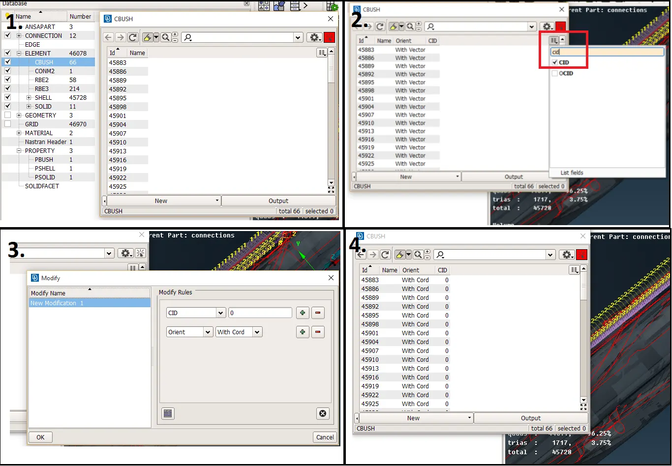
Aligned CBUSH is as follows: