Week 5 - Turbulence modelling challenge

`k-omega` model:In Computational Fludi Dynamics, the k–omega (k–ω) turbulence model is a common two-equation turbulence model, that is used as an approximation for the Reynolds averaged Navier stokes equations (RANS equations). The model attempts to predict turbulence by two partial differential equations for two variables, k and ω, with the first variable being the turbulent kinetic energy (k) while the second (ω) is the specific rate of dissipation (of the turbulence kinetic energy k into internal thermal energy).

`K-epsilon` model:

K-epsilon (k-ε) turbulence model is the most common model used in CFD to simulate mean flow characteristics for turbulent flow conditions. It is a two equation model that gives a general description of turbulence by means of two transport equations (partial differential equations, PDEs). The original impetus for the K-epsilon model was to improve the mixing length model, as well as to find an alternative to algebraically prescribing turbulent length scales in moderate to high complexity flows.

• The first transported variable is the turbulent kinetic energy (k).
• The second transported variable is the rate of dissipation of turbulent kinetic energy (ε).

Spalart Allmaras model:The Spalart–Allmaras model is a one-equation model that solves a modelled transport equation for the kinematic eddy turbulent viscosity. The Spalart–Allmaras model was designed specifically for aerospace applications involving wall-bounded flows and has been shown to give good results for boundary layers subjected to adverse pressure gradients. It is also gaining popularity in turbomachinary applications.

In its original form, the model is effectively a low-Reynolds number model, requiring the viscosity-affected region of the boundary layer to be properly resolved ( y+ ~1 meshes). The Spalart–Allmaras model was developed for aerodynamic flows. It is not calibrated for general industrial flows, and does produce relatively larger errors for some free shear flows, especially plane and round jet flows. In addition, it cannot be relied on to predict the decay of homogeneous, isotropic turbulence.

Reynolds stress equation model (RSM): Also referred to as second moment closures are the most complete classical turbulence model. In these models, the eddy-viscosity hypothesis is avoided and the individual components of the Reynolds stress tensor are directly computed. These models use the exact Reynolds stress transport equation for their formulation. They account for the directional effects of the Reynolds stresses and the complex interactions in turbulent flows. Reynolds stress models offer significantly better accuracy than eddy-viscosity based turbulence models, while being computationally cheaper than Direct Numerical Simulations (DNS) and Large Eddy Simulations.

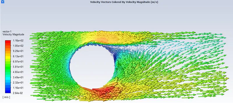
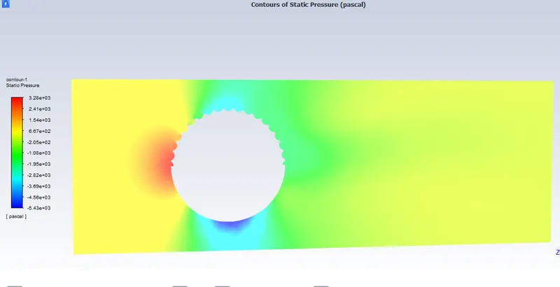
It can be observed that the pressure is high on the left side at the point where the air first encounters the ball. This part, the pressure is the stagnation pressure and hence high values of pressure on this part.

The pressure is higher on the top surface of the ball as compared to the bottom surface. This means that the ball has the tendency to move downward. This is because of the net resultant pressure acting on the ball in the downward direction.

Reasons for the dimples of golf ball:

1) It was observed that in case of a golf ball which is really smooth, it does not travel lot of distance and a rougher ball( a smooth ball which gets old on prolonged usage) travels a lot more distance.

2) To avoid this problem, the gold balls are designed with irregularities in the start and slowly with dimples because of which the turbulence in the flow increases. As a result of this, increase in turbulence, there is higher pressure drag.