Week 5 - Turbulence modelling challenge
TURBULENCE MODELS FOR CFD APPLICATIONS
DNS MODEL
A direct numerical simulation (DNS) is a simulation in computational fluid dynamics (CFD) in which the Navier–Stokes equations are numerically solved without any turbulence model. This means that the whole range of spatial and temporal scales of the turbulence must be resolved. All the spatial scales of the turbulence must be resolved in the computational mesh, from the smallest dissipative scales (Kolmogorov microscales), up to the integral scale { , associated with the motions containing most of the kinetic energy. The Kolmogorov scale,
  , is given by

where  is the kinematic viscosity and
  is the rate of kinetic energy dissipation. On the other hand, the integral scale depends usually on the spatial scale of the boundary conditions.
To satisfy these resolution requirements, the number of points  along a given mesh direction with increments
  , must be

so that the integral scale is contained within the computational domain, and also
so that the Kolmogorov scale can be resolved.
Since

 is the root mean square (RMS) of the velocity, the previous relations imply that a three-dimensional DNS requires a number of mesh points
  satisfying

where  is the turbulent Reynolds number:

Hence, the memory storage requirement in a DNS grows very fast with the Reynolds number. In addition, given the very large memory necessary, the integration of the solution in time must be done by an explicit method. This means that in order to be accurate, the integration, for most discretization methods, must be done with a time step,  , small enough such that a fluid particle moves only a fraction of the mesh spacing in each step. That is,

 is here the Courant number). The total time interval simulated is generally proportional to the turbulence time scale
  given by
\
Combining these relations, and the fact that } must be of the order of , the number of time-integration steps must be proportional to  . By other hand, from the definitions for , and given above, it follows that
and consequently, the number of time steps grows also as a power law of the Reynolds number.
One can estimate that the number of floating-point operations required to complete the simulation is proportional to the number of mesh points and the number of time steps, and in conclusion, the number of operations grows as  .
.
Therefore, the computational cost of DNS is very high, even at low Reynolds numbers. For the Reynolds numbers encountered in most industrial applications, the computational resources required by a DNS would exceed the capacity of the most powerful computers currently available. However, direct numerical simulation is a useful tool in fundamental research in turbulence. Using DNS it is possible to perform "numerical experiments", and extract from them information difficult or impossible to obtain in the laboratory, allowing a better understanding of the physics of turbulence. Also, direct numerical simulations are useful in the development of turbulence models for practical applications, such as sub-grid scale models for large eddy simulation (LES) and models for methods that solve the Reynolds-averaged Navier–Stokes equations (RANS). This is done by means of "a priori" tests, in which the input data for the model is taken from a DNS simulation, or by "a posteriori" tests, in which the results produced by the model are compared with those obtained by DNS.
LES MODEL
Large eddy simulation (LES) is a mathematical model for turbulence used in computational fluid dynamics. It was initially proposed in 1963 by Joseph Smagorinsky to simulate atmospheric air currents,and first explored by Deardorff (1970). LES is currently applied in a wide variety of engineering applications, including combustion, acoustics, and simulations of the atmospheric boundary layer.
The simulation of turbulent flows by numerically solving the Navier–Stokes equations requires resolving a very wide range of time and length scales, all of which affect the flow field. Such a resolution can be achieved with direct numerical simulation (DNS), but DNS is computationally expensive, and its cost prohibits simulation of practical engineering systems with complex geometry or flow configurations, such as turbulent jets, pumps, vehicles, and landing gear.
The principal idea behind LES is to reduce the computational cost by ignoring the smallest length scales, which are the most computationally expensive to resolve, via low-pass filtering of the Navier–Stokes equations. Such a low-pass filtering, which can be viewed as a time- and spatial-averaging, effectively removes small-scale information from the numerical solution. This information is not irrelevant, however, and its effect on the flow field must be modeled, a task which is an active area of research for problems in which small-scales can play an important role, such as near-wall flows, reacting flows, and multiphase flows
An LES filter can be applied to a spatial and temporal field  and perform a spatial filtering operation, a temporal filtering operation, or both. The filtered field, denoted with a bar, is defined as:[9][10]

where  is the filter convolution kernel. This can also be written as
The filter kernel has an associated cutoff length scale  and cutoff time scale
  . Scales smaller than these are eliminated from
  . Using the above filter definition, any field
  may be split up into a filtered and sub-filtered portion, as}
It is important to note that the large eddy simulation filtering operation does not satisfy the properties of a Reynolds operator.
RANS MODEL
The Reynolds-averaged Navier–Stokes equations (or RANS equations) are time-averaged equations of motion for fluid flow. The idea behind the equations is Reynolds decomposition, whereby an instantaneous quantity is decomposed into its time-averaged and fluctuating quantities, an idea first proposed by Osborne Reynolds. The RANS equations are primarily used to describe turbulent flows. These equations can be used with approximations based on knowledge of the properties of flow turbulence to give approximate time-averaged solutions to the Navier–Stokes equations. For a stationary flow of an incompressible Newtonian fluid, these equations can be written in Einstein notation in Cartesian coordinates as:

The left hand side of this equation represents the change in mean momentum of a fluid element owing to the unsteadiness in the mean flow and the convection by the mean flow. This change is balanced by the mean body force, the isotropic stress owing to the mean pressure field, the viscous stresses, and apparent stress  owing to the fluctuating velocity field, generally referred to as the Reynolds stress. This nonlinear Reynolds stress term requires additional modeling to close the RANS equation for solving, and has led to the creation of many different turbulence models. The time-average operator
  is a Reynolds operator.
The basic tool required for the derivation of the RANS equations from the instantaneous Navier–Stokes equations is the Reynolds decomposition. Reynolds decomposition refers to separation of the flow variable (like velocity  ) into the mean (time-averaged) component }
 ) and the fluctuating component (). Because the mean operator is a Reynolds operator, it has a set of properties. One of these properties is that the mean of the fluctuating quantity is equal to zero
  . Thus,
 , where
  is the position vector. Some author prefer using
  instead of
  for the mean term (since an overbar is sometimes used to represent a vector). In this case, the fluctuating term is represented instead by {\displaystyle u}. This is possible because the two terms do not appear simultaneously in the same equation. To avoid confusion, the notation
  will be used to represent the instantaneous, mean, and fluctuating terms, respectively.
The properties of Reynolds operators are useful in the derivation of the RANS equations. Using these properties, the Navier–Stokes equations of motion, expressed in tensor notation, are (for an incompressible Newtonian fluid):


where is a vector representing external forces.
Next, each instantaneous quantity can be split into time-averaged and fluctuating components, and the resulting equation time-averaged,to yield:


The momentum equation can also be written as,

On further manipulations this yields,

where, }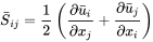 is the mean rate of strain tensor.
Finally, since integration in time removes the time dependence of the resultant terms, the time derivative must be eliminated, leaving:

The time evolution equation of Reynolds stress is given by:

This equation is very complicated. If  is traced, turbulence kinetic energy is obtained. The last term
  is turbulent dissipation rate. All RANS models are based on the above equation.
Spalart Adamas Model
The Spalart–Allmaras model is a one-equation model that solves a modeled transport equation for the kinematic eddy turbulent viscosity. The Spalart–Allmaras model was designed specifically for aerospace applications involving wall-bounded flows and has been shown to give good results for boundary layers subjected to adverse pressure gradients. It is also gaining popularity in turbomachinery applications.
In its original form, the model is effectively a low-Reynolds number model, requiring the viscosity-affected region of the boundary layer to be properly resolved ( y+ ~1 meshes). The Spalart–Allmaras model was developed for aerodynamic flows. It is not calibrated for general industrial flows and does produce relatively larger errors for some free shear flows, especially plane and round jet flows. In addition, it cannot be relied on to predict the decay of homogeneous, isotropic turbulence.It solves a transport equation for a viscosity-like variable  . This may be referred to as the Spalart–Allmaras variable.
The turbulent eddy viscosity is given by







The rotation tensor is given

where d is the distance from the closest surface and  is the norm of the difference between the velocity at the trip (usually zero) and that at the field point we are considering.
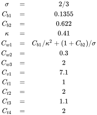
The constants are
K-Epsilon Model
K-epsilon (k-ε) turbulence model is the most common model used in Computational Fluid Dynamics (CFD) to simulate mean flow characteristics for turbulent flow conditions. It is a two-equation model that gives a general description of turbulence by means of two transport equations (PDEs). The original impetus for the K-epsilon model was to improve the mixing-length model, as well as to find an alternative to algebraically prescribing turbulent length scales in moderate to high complexity flows.
- The first transported variable is the turbulent kinetic energy (k).
- The second transported variable is the rate of dissipation of turbulent kinetic energy (ε).
The exact k-ε equations contain many unknown and unmeasurable terms. For a much more practical approach, the standard k-ε turbulence model (Launder and Spalding, 1974[3]) is used which is based on our best understanding of the relevant processes, thus minimizing unknowns and presenting a set of equations which can be applied to a large number of turbulent applications.
For turbulent kinetic energy k

For dissipation

| Rate of change of k or ε in time + Transport of k or ε by advection = Transport of k or ε by diffusion + Rate of production of k or ε - Rate of destruction of k or ε |
where
 represents velocity component in corresponding direction
 represents component of rate of deformation
 represents eddy viscosity

The equations also consist of some adjustable constants  ,
,  ,
,  and
and  . The values of these constants have been arrived at by numerous iterations of data fitting for a wide range of turbulent flows. These are as follows:


Realizable k- ε Model:
An immediate benefit of the realizable k-ɛ model is that it provides improved predictions for the spreading rate of both planar and round jets. It also exhibits superior performance for flows involving rotation, boundary layers under strong adverse pressure gradients, separation, and recirculation. In virtually every measure of comparison, Realizable k-ɛ demonstrates a superior ability to capture the mean flow of the complex structures.
RNG K epsilon Model
There are a number of ways to write the transport equations for k and , a simple interpretation where bouyancy is neglected is


where 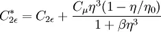
and  and
and 
With the turbulent viscosity being calculated in the same manner as with the standard k-epsilon model.
Constants
It is interesting to note that the values of all of the constants (except  ) are derived explicitly in the RNG procedure. They are given below with the commonly used values in the standard k-epsilon equation in brackets for comparison:
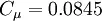 (0.09)
 (1.0)
(1.0) (1.30)
 (1.44)
 (1.92)

K- OMEGA MODEL
In computational fluid dynamics, the k–omega (k–ω) turbulence model is a common two-equation turbulence model, that is used as an approximation for the Reynolds-averaged Navier–Stokes equations (RANS equations). The model attempts to predict turbulence by two partial differential equations for two variables, k and ω, with the first variable being the turbulence kinetic energy (k) while the second (ω) is the specific rate of dissipation (of the turbulence kinetic energy k into internal thermal energy).Standard (Wilcox) k–ω turbulence model
The eddy viscosity νT, as needed in the RANS equations, is given by: νT = k/ω, while the evolution of k and ω is modelled as:

K OMEGA SST MODEL
Menter's Shear Stress Transport turbulence model, or SST, is a widely used and robust two-equation eddy-viscosity turbulence model used in Computational Fluid Dynamics. The model combines the k-omega turbulence model and K-epsilon turbulence model such that the k-omega is used in the inner region of the boundary layer and switches to the k-epsilon in the free shear flow.


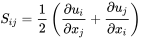
Variable Definition


}
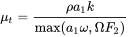





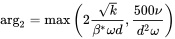
Constants
 , }
, } ,
, 
 ,
,  ,
, 
 ,
, 
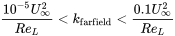
Far Field
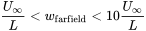
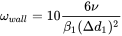
Boundary/Wall Conditions

GOLF BALL SIMULATION
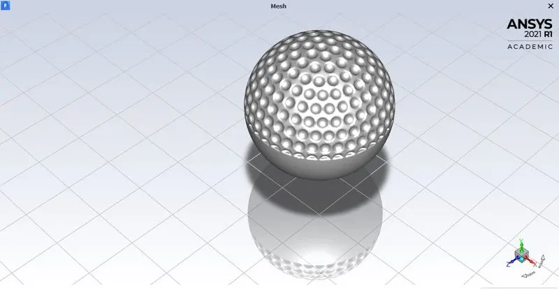
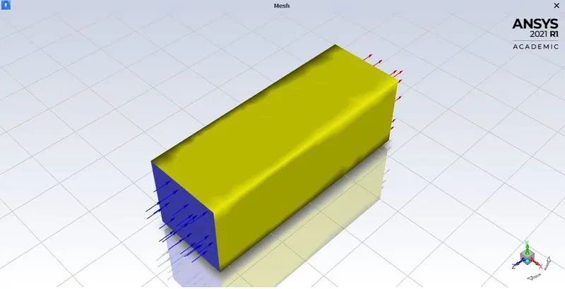
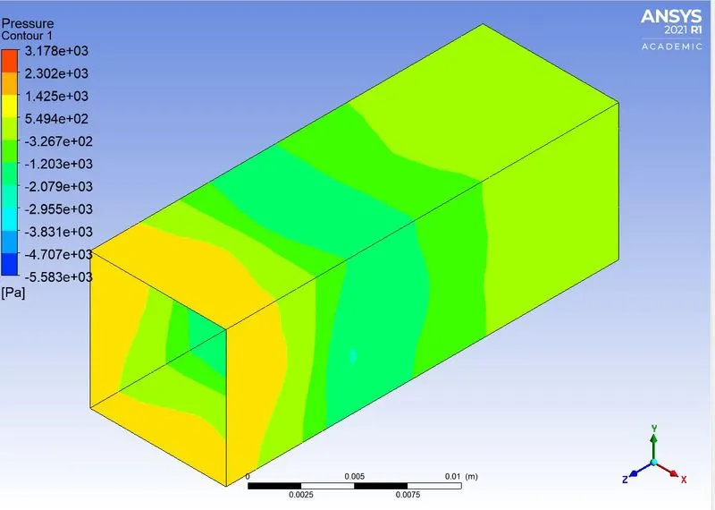
The geometry file shows a golf ball within the enclosure to perform an aerodynamic simulation.
Setup
- Solver - Pressure based
- Solver state - steady
- Fluid - Air
- Inlet Velocity = 60m/s
- Outlet Pressure = 0 Pa
- Wall - Wall Boundary
- Turbulence Model - K-Omega
Results
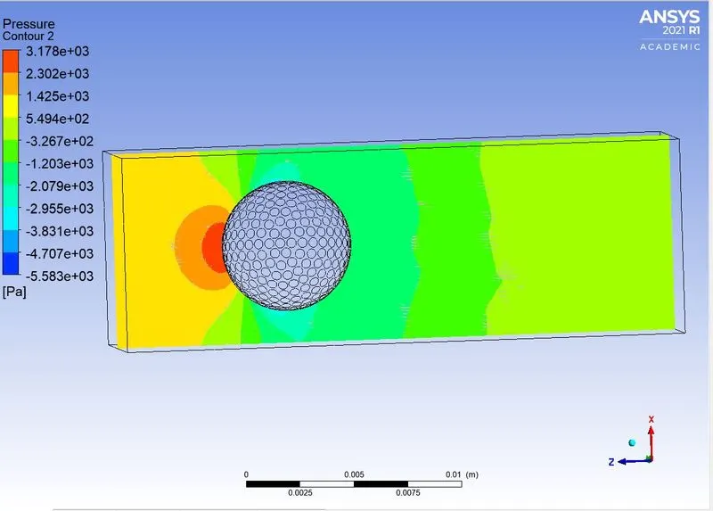
Pressure contour
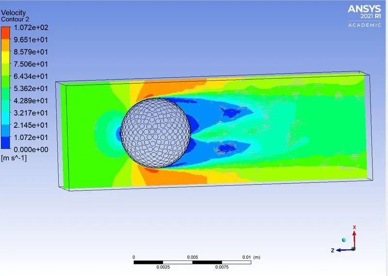
Velocity Contours
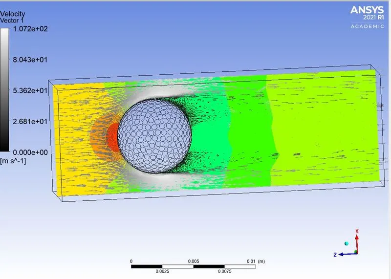
The vector plot shows the recirculation zone which causes a drop in pressure after the flow. The ball will curve away from the direction of the wind.
CONCLUSION
- The golf ball aerodynamics is conducted
- Velocity vector plot shows the recirculation zones
- The wake region can be clearly visualized.