Project Report

Rayleigh Taylor Instability

Introduction

The Rayleigh–Taylor instability, also called RT instability is an instability at the interface between two fluid of different densities, when the lighter fluid is pushing the heavier fluid. The flow or turbulent mixing is the consequence of lowering the potential energy of the system. The initial configuration has higher potential energy than the later.

Various types of instabilities and practical models based on mathematical analysis of RT Instabilities are as follows: -

Kelvin-Helmholtz Instability

Visible at interface of two different fluid, when there is velocity difference or in a continuous fluid when there is velocity shear. This theory predicts the onset of instability and transition to turbulent flow within fluids of different densities moving at various speeds. The common example is when the wind bows at a water surface, the instability is manifested as waves.

Richtmyer-Meshkov Instability (RM Instability)

The Richtmyer–Meshkov instability or RMI occurs when two fluids of different density are impulsively accelerated. The phenomenon occurs by passage of shockwave. The development of the instability begins with small amplitude perturbations which initially grow linearly with time, followed by a nonlinear regime with bubbles appearing in the case when light fluid penetrates a heavy fluid, and with spikes appearing when heavy fluid penetrates a light fluid. Finally, a chaotic regime is reached and the two fluids mixes.

Plateau-Rayleigh Instability

The Plateau–Rayleigh instability, also called Rayleigh instability, explains why and how a falling stream of fluid breaks up into smaller packets with the same volume but less surface area. The driving force of the phenomenon is that liquids, by virtue of their surface tensions, tend to minimize their surface area.

K-L Turbulence Model

It’s a 2-equation turbulence model proposed to simulate RT and RM instabilities. K is the turbulent kinetic energy and L represents turbulent eddy scale length. The model uses evolutionary equations to describe dominant eddies characteristics length in mixing zones and energy density.

Objective

The scope of the work is to figure out difference between results of phase concentration of different fluid regions with the variation in mesh size.

The simulation will also focus on studying the effect of varying density among mixing fluid on the interface instability.

Difference in transient vs steady state solution of the given phenomenon will also be discussed.

Rayleigh Taylor instability simulation

In order to achieve the above objective 4 cases has been designed as follows: -

Case 1 – Baseline Mesh Simulation

In this case, coarse mesh is used to simulate the physics. The mesh may or may not be sufficient to capture the minute results like instability of the separation layer. The sole purpose of running a successful base line simulation is setting up the problem for simulating the phenomenon with least computational resource, over which it can be improved further. The cell size is 0.0005m in this case.

Case 2 – Refined Mesh (Air Water interface)

In this case, fine mesh is used to simulate the physics. The mesh density has been increased to sufficiently capture the phenomenon in detail. Element size in this case has been reduced to 0.00005m. The fluids in this case are air and water.

Case 3 – Refined Mesh (Water and User Material)

In this case, previously used fine mesh has been used to simulate the RT instability. The fluid media is Water and a user defined fluid. The density of user defined material is 400Kg/m3 and a viscosity of 0.001Kg/(m-s). The case in comparison with case 2 will help us in observing difference with Atwood number on the interface instability.

Case 4

In this case steady state simulation of Air and water media is done to observe the difference in results.

Geometry

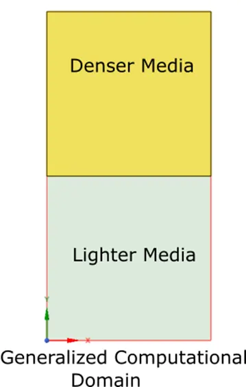
For computational simplicity, the interface stability is modelled and solved in 2D domain. Square shaped domain of both media is stacked on top of another to simulate the gravitational pull and buoyant push of the two media.

Meshing

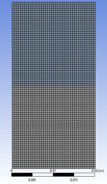
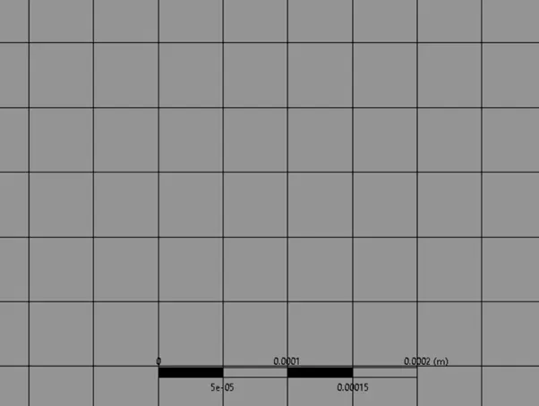
The domain is divided into 2 cell zones, the cell size is the controlling factor in meshing. The final refined mesh’s element size is of 0.00005m whereas the baseline mesh has element size of 0.0005m.

Solver Settings

Solver

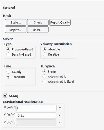
Pressure based solver has been used with absolute velocity formulation. Since the simulation is dependent on gravitational forces, gravity has been enabled in the solver.

Viscous Model has been chosen to be of Laminar nature.

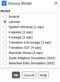
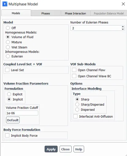
Since we are dealing with buoyant forces, we need to have multiphase model. Volume of fluid has been chosen as the multiphase model in this study with implicit volume fraction simulation.

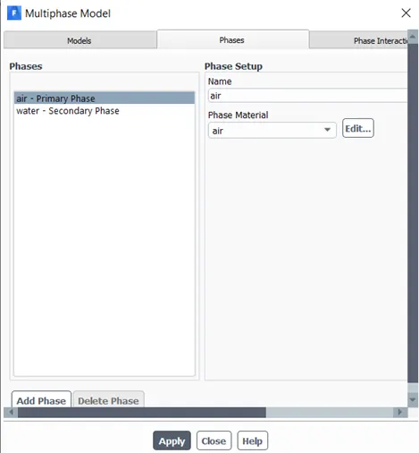
The phases have been configured as per the case, switching primary and secondary phases with different fluid particles.

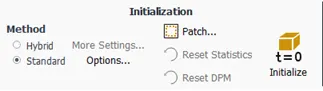
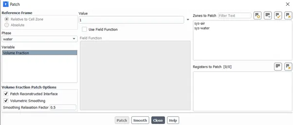
Later the simulation is initialized, with standard method. Following initialization, the cell zones are patched different phases.

Time Step

As stated in the objective, the simulation has been done as to compare the steady as well as transient state too, so the instability results are interpreted in transient state with time step size of 0.001s and total time step of 6000.

Results and Discussions

The evolution of the RT Instability follows four main stages.

• In beginning stage, the perturbation amplitudes appear small as compared to their wavelengths, the equations of motion can be linearized, resulting in exponential instability growth. In the beginning of this stage, a sinusoidal initial perturbation retains its sinusoidal shape, but in ending of first stage, when non-linear effects begin to appear, one observes the beginnings of the formation of the mushroom-shaped spikes and bubbles.
• The growth of the mushroom structures continues in the second stage, resulting in a growth rate that is approximately constant with time. At this point, nonlinear terms in the equations of motion is evident.
• The spikes and bubbles then begin to interact with one another in the third stage. Bubble merging takes place, where the nonlinear interaction of mode coupling acts to combine smaller spikes and bubbles producing larger ones. Also, bubble competition takes places, where spikes and bubbles of smaller wavelength that have become saturated are enveloped by larger ones that have not yet saturated.
• This eventually develops into a region of turbulent mixing, which is the fourth and final stage in the evolution.

Case 1

Case 2

Case 3

It is quite evident fromt the above results that, for case with water and user defined fluid, the mixing process seems larger, also the slush region us much wider as compared with water and air simulation. The phenomenon can be corelated with atwood number.

Atwood Number is defined as,

`A = {rho_1 - rho_2}/{rho_1 + rho_2}`

Where as,

`rho_1` = Density of heavy fluid

`rho_2 =` Density of lighter fluid

Atwood number is lesser for interface with less difference in densities.

Atwood Number for Water Air Interface:-

`A = {998.2 - 1.225}/{998.2 + 1.225}`

`A = 0.998`

Atwood Number for Water and User defined Interface:-

`A = {998.2 - 400}/{998.2 + 400}`

`A = 0.428`

As stated earlier, for less difference in density the Atwood Number is lesser. When the Atwood number is small, the mixing is delayed as compared to the prior.

The penetration distance of heavy fluid bubbles into the light fluid is a function of acceleration time scale `At^2`, where A is the Atwood Number, g is the gravitational acceleration and t is the time.

With the increase in the Atwood number, the stabilization effect of initial density stratification decreases, and the instability caused by the expansion-compression effect becomes more significant. The flow structures of bubbles and spikes are quite different at medium Atwood number. The effect of compressibility on the bubble velocity is strong at large At. The bubble height is approximately a quadratic function of time at potential flow growth stage.

Steady state solution to the problem will be unable to investigate the instability as it is a transient phenomenon. Though the simulation has been carried out in steady state and the result has been plotted below.

The simulation was run for 1000 iteration, It needs to run for a bit longer duration of time for the phases to seperate out.

References

Luo, Tengfei, et al. "Effects of compressibility and Atwood number on the single-mode Rayleigh-Taylor instability." Physics of Fluids 32.1 (2020): 012110.