Week 5 - Rayleigh Taylor Instability

Rayleigh Taylor instability is the instability of an interface between two fluids of different densities which occurs when the lighter fluid is pushing the heavier fluid. Water suspended atop oil is an everyday example of Rayleigh–Taylor instability, and it may be modeled by two completely plane-parallel layers of immiscible fluid, the more dense on top of the less dense one and both subject to the Earth's gravity.

Practical CFD models that have been based on mathematical analysis of Rayleigh Taylor waves...

1. Kelvin-Helmholtz instability
2. Richtmyer-Meshkov instability
3. Plateau-Rayleigh instability

Kelvin-Helmholtz instability- This instability typically occurs when there is velocity shear in a single continuous fluid or when there is a velocity difference across the interface between two fluids.

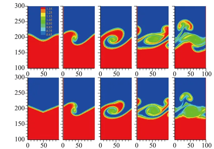
Richtmyer-Meshkov instability- This occurs when two fluids of different density are impulsively accelerated. Normally this is by the passage of a shock wave.The development of the instability begins with small amplitude perturbations which initially grow linearly with time. This is followed by a nonlinear regime with bubbles appearing in the case of a light fluid penetrating a heavy fluid, and with spikes appearing in the case of a heavy fluid penetrating a light fluid. A chaotic regime eventually is reached and the two fluids mix. This instability can be considered the impulsive-acceleration limit of the Rayleigh Taylor Instability.

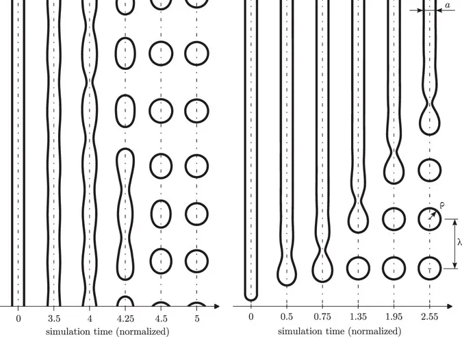
Plateau-Rayleigh instability- This instability explains why and how a falling stream of fluid breaks up into smaller packets with the same volume but less surface area.

2. Perform the Rayleigh Taylor instability simulation for 2 different mesh sizes with the base mesh being 0.5 mm

For this simulation, we create 2 components of Air & water.

1) Sketch 2 rectangles of size 20x20 mm, lower one of air & upper one for water.

2) Create a baseline mesh of 0.5 mm.

3) In setting up physics select Laminar model

4) In Solver select pressure-based and assign time as transient (non-steady state)

5) Material selection: 1) water & air

6) Properties of Material:

for air: density= 1.22 kg/m^3

viscosity= 0.0000181 kg/m.s

for water: density= 997 kg/m^3

viscosity= 0.0000890 kg/m.s

7) Enable gravity= -9.81 m/s^2

8) select volume of fluid method & number of phases are 2, one is water & one is air.

9) select implicit method.

10) Rename phases as air & water.

11) Standard initialization.

12) Then patch the model by selecting water as phase and value of water to be kept 1 and for air it has to be 0.

13) Create phase contour

14)Create animation as per time step

15) assign time step size 0.005s & number of time steps 1000.

Animation for mesh size 0.5 mm

https://drive.google.com/file/d/130ScA6HPpMJ181Ds1oOKGI1FLASkweq3/view?usp=share_link

Animation for mesh size 0.3 mm

https://drive.google.com/file/d/1VEqlfolcbnJwaSEka2cgiPuFlZnqUgZF/view?usp=share_link

Animation for mesh size 0.2 mm

https://drive.google.com/file/d/15DK57EMhAW9Hdcmy6YZGgTtYMk6hOwlu/view?usp=share_link

Comparison of simulation with three different mesh size.

1) In the animation with mesh size 0.5 mm, flow pattern is not clearly visible, whereas the flow pattern and bubble formation is clearly visible in animation with 0.2 mm. This shows that as the mesh gets refined, the bubble formation and flow pattern gets clearly visible.

2) The time required for calculation of simulation for refined mesh is more than that of bigger mesh size.

why a steady-state approach might not be suitable for these types of simulation,

In steady state approach, time is constant, Hence it cannot be used for simulation fo taylor instability as the flow pattern caused due to instability between to surface can be observed with respect to time. So steady state approach cannot be used in simulation of Taylor instability equation.

Animation for simulation with water and user-defined material(density = 400 kg/m³, viscosity = 0.001 kg/m-s) for refined mesh.

https://drive.google.com/file/d/1pBmgSuNnXhGMYJ-1BaMQnOTDK4IRO1Bk/view?usp=share_link

Atwood Number :

The Atwood number is a dimensionless number in fluid dynamics used in the study of hydrodynamic instabilities in density-stratified flows. The Atwood number equals the ratio of the difference in mass densities to their sum.

Case 1 (For air and water)

Atwood Number = 0.9975

Case 2 (For water and user defined material of density = 400 kg/m³, viscosity = 0.001 kg/m-s):

Atwood Number = 0.4273

How the variation in Atwood number in the above two cases affects the behavior of the instability ?

1) Rayleigh–Taylor instability at high Atwood numbers is characterized by rapid development of instability due to the increasing growth rates and higher velocities of spike fronts, larger asymmetry in the mixing region, denser interactions in the non-linear phase, and changes in bubble and spike.

2) So the instabiliy is raidly developed in Case 1 where the Atwood no. is highest and is found to be slowly developing in Case 2