Week 5 - Rayleigh Taylor Instability

Rayleigh–Taylor instability

John William Strutt, 3rd Baron Rayleigh was a British mathematician and physicist who made extensive contributions to science.

Sir Geoffrey Ingram Taylor was a British physicist and mathematician, and a major figure in fluid dynamics and wave theory.

Rayleigh–Taylor instability is an instability results from heavier fluid being pushed by lighter fluid. Some of the examples are volcanic eruptions, atmospheric nuclear explosions, supernova explosions, plasma fusion reactors, inertial confinement fusion. Water suspended on atop oil is an everyday example of Rayleigh-Taylor instability.

Single phase fluid flows pre dominate the majority of the time when applied to pipe flow and other conveying media. Multiphase flows have recently been introduced and are gaining popularity in industrial development applications.

Multiphase flow is the interactive flow of two or more distinct phases with common interfaces. Each phase, representing a volume fraction (or mass fraction) of solid, liquid, or gaseous matter, has its own properties, velocity, and temperature. In the chemical industry, nuclear industry, manufacturing facilities, and product agitator mixing, multiphase flows are used.

In the multi phase model there are two approaches

1. Euler-Lagrange approach
2. Euler-Euler approach

For multiphase flows, the Lagrangian-Eulerian (LE) method is used. The LE method is based on a statistical description of the dispersed phase in terms of a stochastic point process, which is connected with a statistical representation of the carrier fluid phase in terms of an Eulerian statistical representation.

The fluid phase is handled as a continuum by solving the Navier-Stokes equations, whereas the dispersed phase is solved by tracking a large number of particles, bubbles, or droplets through the estimated flow field. Momentum, mass, and energy can be exchanged between the dispersed and fluid phases.

Euler–Euler (EE) models describe both the fluid and the particulate phase with transport equations on a globally fixed coordinate system—particles are not tracked in space and time. Instead, the distribution of particle phase properties (e.g., speed, size, composition, etc.) is considered. There are three modes of approach namely VOF model, mixture model and Euler model.

Tailor's unstable interface is associated with a complex phenomenology. Spikes, curtains, and bubbles are examples of this.

Helmholtz instability on the spike side, bubble competition resulting in amalgamation, droplet formation, entrainment, and turbulent mixing, and a probable chaotic limit with a fractionized interface.

Atwood Number:

The Atwood number is a dimensionless number in fluid dynamics used in the study of hydrodynamic instabilities in density-stratified flows. The Atwood number equals the ratio of the difference in mass densities to their sum.

ρ1- Fluid density(Water) ρ2- fluid density of lighter fluid(Air/UDM)

Model Approach:

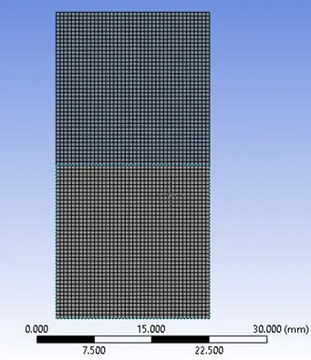
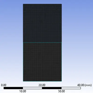
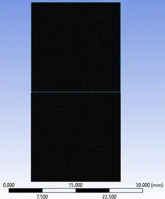
The simulation method is simple; it is a two-dimensional analysis with two surfaces connected by an interface. The solution methodology is designed with simulation in mind. The simulation will take place in the following mesh size of 0.5, 0.25, and 0.125 mm respectively.

As long as two fluids are present, multiphase simulation will be performed. We will use the Volume of Fluid approach, which is well known for sloshing simulations, for the multiphase. We previously discussed the existence of a phase interface between two immiscible liquids. It is critical to develop a mechanism that accurately predicts the fluid interface's kinematic motion in order to monitor it.

The moving grid method, marker particle methods, and the VOF method are the most commonly used interface tracking methods in FLUENT. To treat small free surface deformations, the moving grid or adaptive grid approach is commonly used. Without changing the mesh topology, this method cannot handle large deformation problems.

Geometry:

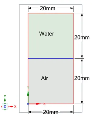
Here we are designed the model in space claim with the below detail dimension in XY plane. It’s a 2D drawing. Pull tool is used to create a surface of the given fluid. Share tool is used to create a conformal mesh between the boundary between water and air.

Mesh:

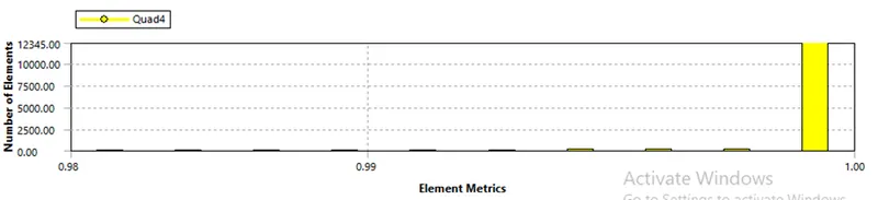
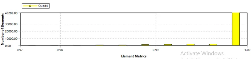
Default mesh will be generated first them mesh size is changed. Here in my work I used to made simulation by three types of mesh sizes, i.e. 0.5, 0.25 and 0.125mm mesh respectively.

	Mesh 0.5	Mesh 0.25	Mesh 0.125
Nodes	3321	13041	51681
Elements	3200	12800	51200

Set up:

Boundary condition

Solver	Steady state, Pressure Based
Turbulence(viscosity)	Laminar
Gravity	On (-9.81 in Y Direction)
Multiphase Model	Volume of Fluid
Material	Air, Water, User Defined Material
Phase 0	Air, UDM
Phase1	Water
Initialization	Standard
Air Density & Viscosity	1.225 kg/m3, 1.7894e-05 kg/m-s
Water density	998.2 kg/m3
User defined Material Density & Viscosity	400 kg/m3 & 0.001 kg/m-s
Atwood Number	0.9975
Atwood Number(UDM)	0.4278
Patch 0	Air, UDM
Patch 1	Water

While steady-state simulation is possible, the VOF model is most typically utilised to solve time-dependent problems. A steady state simulation of the VOF model makes sense only when our answer is independent of the beginning conditions and provides precise inflow and outflow boundary conditions for each phase. A steady state solution is used when results are required at the end of a time step and no intermediate phase outcomes are required. In the event of instability, it is critical to guarantee that the volume fraction is a function of time since it will change over time.

Mesh

Mesh 0.5

Mesh 0.25

Mesh 0.125

Results:

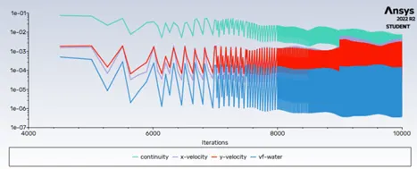
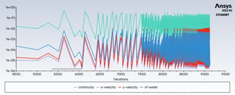
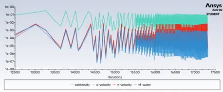
Residuals

Air	User Defined Material

Volume Fraction

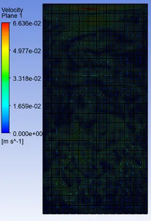
Velocity

Pressure

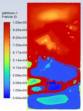
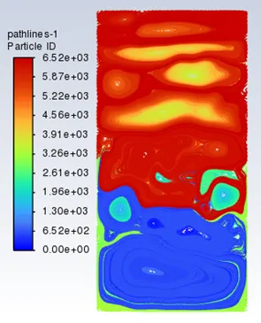
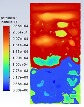
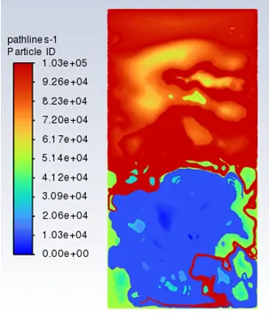
Path lines

Mesh 0.5	Mesh 0.25	Mesh 0.125
User defined Material

Results & Conclusion:

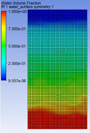
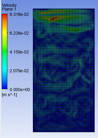
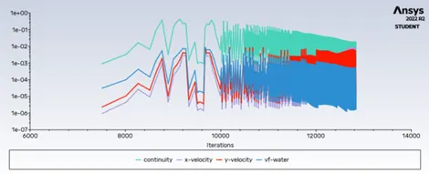
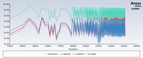
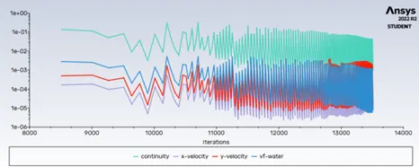
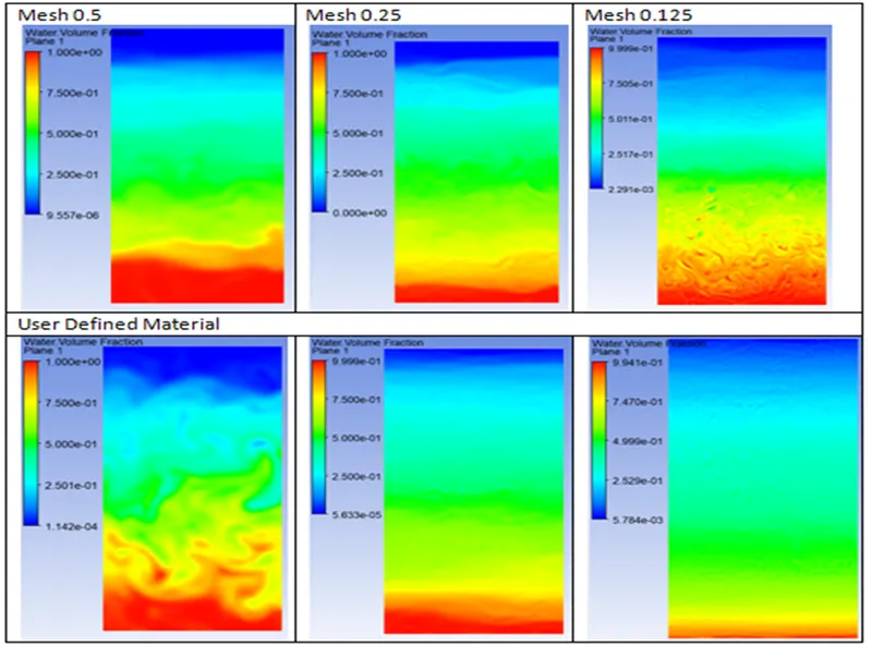
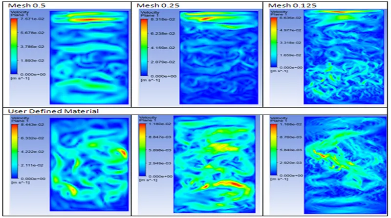
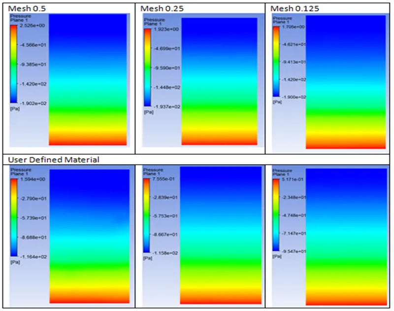
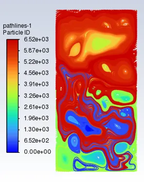
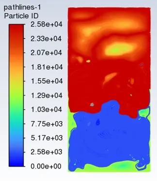
• The volume fraction for water drops sooner in the Default mesh configuration, and as the mesh size decreases, the decline advances in time. This means that as the number of elements and nodes increases, we capture flow dynamics better. As a result, we may assert that mesh size influences how hydrodynamic instability convergence occurs.
• When the heavier fluid accelerates into the lighter fluid, the acceleration is reduced. The Atwood Number, which was mentioned in the study, is capable of quantifying this.
• We utilized an implicit technique to address the problem because the fluid's instability is significantly dependent on small time steps.
• Furthermore, the implicit technique involves more computational work at each time step size, resulting in better numerical stability.
• As the mesh size goes on decreases the number of iterations to converge goes on increases and as the Atwood number decreases for user-defined material the number of iterations decreases.

Animation:

Mesh 0.5

Mesh 0.25

Mesh 0.125

0.5-https://drive.google.com/file/d/1bcVNmaBVFwdcvzDc-x0MVo9R5WIRMrer/view?usp=share_link

0.25- https://drive.google.com/file/d/19vbFL5_rNtCFmzztfdBdaNS9bXO9BXru/view?usp=share_link

0.125- https://drive.google.com/file/d/1yJM8n73iJ67C-gMw4tyOsj9gvf_v_6pe/view?usp=share_link

User-defined Material

0.5-https://drive.google.com/file/d/1NZa-eAdUjlZRr_hDuTCEqFuq_sGSwoW5/view?usp=share_link

0.25-https://drive.google.com/file/d/13wf0OEKfaRTHsraIaQWaFP-1v6slvBjW/view?usp=share_link

0.125-https://drive.google.com/file/d/1z45tGirBKXsfZxyQaSX3jxZe1A1hoU6Q/view?usp=share_link