Week 5 - Rayleigh Taylor Instability

ANALYSIS OF INSTABILITY IN TWO FLUID SYSTEM USING RAYLEIGH TAYLOR METHOD

INTRODUCTION:

The Rayleigh-Taylor instability is a fluid dynamic instability that occurs when a fluid with a lower density is placed below the fluid with a higher density. It can be described mathematically using the Rayleigh-Taylor equation, which is a partial differential equation that describes the evolution of the fluid interface.

One practical application of the Rayleigh-Taylor instability is in the analysis of fluid-structure interactions, such as the motion of a submerged object or the behavior of a fluid-filled container subjected to external forces.

In the field of computational fluid dynamics (CFD), there are several models that have been developed to simulate the Rayleigh-Taylor instability, including:

1. The level set method: This is a numerical technique used to track the evolution of the fluid interface. It involves representing the interface as a surface in space, and using partial differential equations to evolve the surface over time.

2. The volume of fluid (VOF) method: This method involves tracking the volume fraction of each fluid within a computational domain. It can be used to simulate the mixing of two fluids, as well as the motion of a fluid-filled object.

3. The front tracking method: This method involves tracking the motion of discrete fluid elements, or "fronts," as they move through the computational domain. It is often used to simulate complex fluid flows, such as those involving shock waves or free surface flows.

Overall, the choice of model will depend on the specific application and the level of detail required in the simulation.

The volume of fluid (VOF) method involves solving a partial differential equation (PDE) to update the volume fractions of each fluid within the computational domain. The VOF equation can be written as follows:

∂φ/∂t + ∇ . (φu) = 0

Where:

φ: Volume fraction of a particular fluid

t: Time

u: Velocity vector of the fluid

∂/∂t: Time derivative

∇: Del operator

To solve this equation numerically, we can discretize the computational domain into a grid of cells, and use finite difference methods to approximate the derivatives. For example, we can use the forward Euler method to approximate the time derivative as follows:

φ(t + Δt) = φ(t) + ∂φ/∂t * Δt

Where Δt is the time step.

APPLICATIONS:

The Rayleigh-Taylor instability method is a widely-used technique for studying fluid instabilities in a variety of contexts. Some examples of areas where this method has been applied include:

• Rocket propulsion systems: The Rayleigh-Taylor instability can occur in the exhaust plume of a rocket, leading to mixing between the exhaust gasses and the surrounding air. By studying this instability, engineers can better understand the effects of the rocket exhaust on the acceleration of the vehicle and optimize the design of the rocket nozzle to minimize mixing.

• Volcanic fumes dispersion: The dispersion of volcanic fumes into the atmosphere can be affected by the Rayleigh-Taylor instability, as the denser fumes mix with the lighter air. By studying this instability, researchers can better understand the transport and dispersion of volcanic gases and develop models to predict their behavior.

• Effects of heavy explosions: The Rayleigh-Taylor instability can also be induced by the shock waves produced by heavy explosions, such as nuclear blasts. By studying this instability, researchers can better understand the dynamics of the explosion and the movement of gases and other materials that are produced.

• Cooling of combustible fuels: In some applications, it may be necessary to cool a combustible fuel by using another fluid that is made to flow over the fuel. The Rayleigh-Taylor instability can occur at the interface between the two fluids, and by studying this instability, engineers can better understand the heat transfer and mixing processes that occur.

• Petroleum industry: The flow of fuels in the petroleum industry can be affected by the Rayleigh-Taylor instability, particularly in storage tanks and pipelines. By studying this instability, researchers can better understand the behavior of the fluids and develop strategies to minimize mixing and improve the efficiency of the system.

There are many other areas where the Rayleigh-Taylor instability method has been applied, including in the biomedical and chemical engineering fields. This method is a powerful tool for studying fluid instabilities and understanding the dynamics of fluids in various contexts.

PRACTICAL CFD MODELS:

The smoothed particle hydrodynamics (SPH) model, single fluid method, two fluid method, and turbulence method are all examples of practical CFD models that have been developed to simulate fluid dynamics and fluid instabilities.

1. Smoothed particle hydrodynamics (SPH) model: The SPH model is a meshless numerical technique that is used to simulate the motion and deformation of fluids and solids. It involves representing the fluid or solid as a set of discrete particles, each of which is assigned a set of physical properties (e.g., mass, velocity, density). By solving the governing equations of motion (e.g., the Navier-Stokes equations) for each particle and using a smoothing kernel to interpolate the physical properties of the particles, it is possible to simulate the motion and deformation of the fluid or solid.

2. Single fluid method: The single fluid method is a technique for simulating the motion of a single fluid within a computational domain. It involves solving the governing equations of fluid motion (e.g., the Navier-Stokes equations) for the single fluid and using appropriate boundary conditions to model the interactions of the fluid with the surrounding environment.

3. Two fluid method: The two fluid method is a technique for simulating the interaction of two fluids within a computational domain. It involves solving the governing equations of fluid motion separately for each fluid and using appropriate boundary conditions to model the interactions between the two fluids.

4. Turbulence method: The turbulence method is a technique for modeling the turbulent flow of fluids, which involves the presence of small-scale, unsteady motions within the fluid. There are many different approaches to modeling turbulence, including the use of empirical models, statistical models, and computational fluid dynamics (CFD) models.

AIM: To study the fluid instability that occurs when two fluids with different densities interact within a single control volume, one can use the Rayleigh-Taylor instability method. In this method, the fluid with a lower density is placed below the fluid with a higher density. This configuration is known as the "non-inverted" configuration, as the denser fluid is typically assumed to be at the top and the lighter fluid is assumed to be at the bottom. The external force that drives the instability can be any type of force that acts on the fluids, such as gravity, acceleration, or pressure gradients. By studying the evolution of the fluid interface over time, it is possible to understand the dynamics of the instability and how it affects the behavior of the fluids.

I used ANSYS FLUENT commercial CFD code

MODELLING: By using SPACECLAIM tool created model.

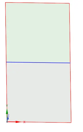
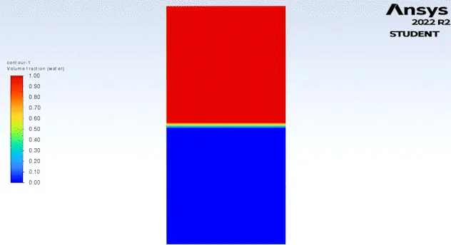
To study the Rayleigh-Taylor instability using computational fluid dynamics (CFD), a geometry with the following dimensions and properties had created:

• The upper domain is a 20x20mm rectangular region filled with water.
• The lower domain is a 20x20mm rectangular region filled with air.
• The two domains are separated by an interface, which can be represented using a shared topology to allow for the exchange of information between the two domains.

MESHING: Generated mesh on the following conditions.

Element size: 0.5 mm.

Obtained Results:

Elements: 3200.

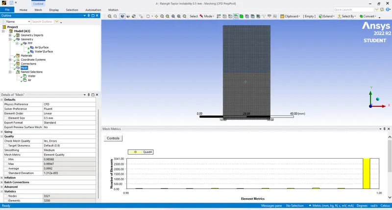
Quality of the mesh is checked and found as satisfactory in nature.

PHYSICS SETUP:

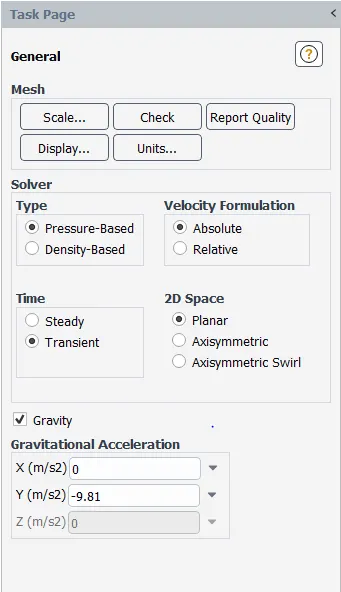
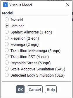
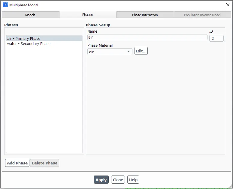
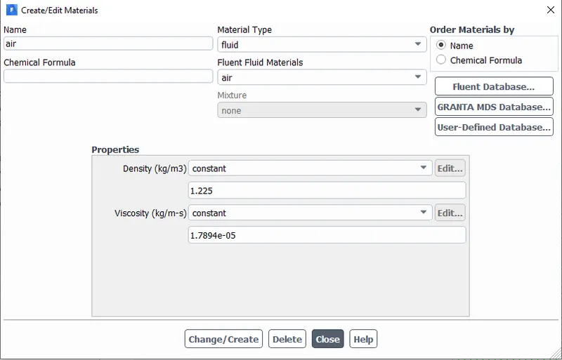
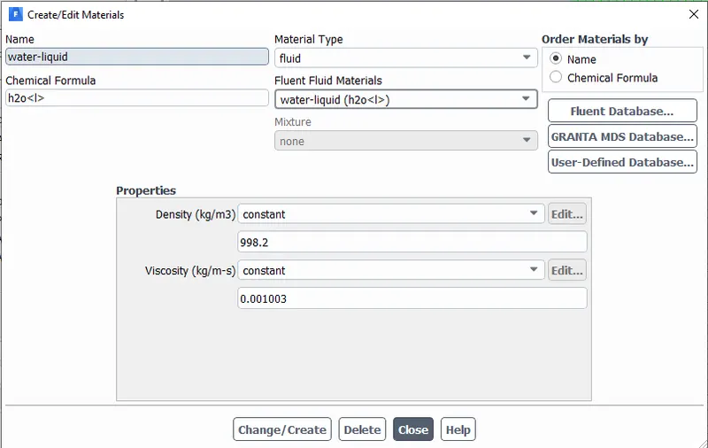
A computational domain was created with two regions: an upper region filled with water and a lower region filled with air. The two regions were separated by an interface, which was represented using a shared topology. The flow conditions were specified as laminar, and gravity forces were applied to the fluids. The material properties of air and water were assigned to the two regions.

A transient-based solver was used to simulate the evolution of the fluids over time. The time step size was set to 0.005 seconds, and the number of time steps was set to 1000. The solution was initialized using the standard initialization method, and the surfaces of the two regions were patched with the appropriate values (water=1, air=0).

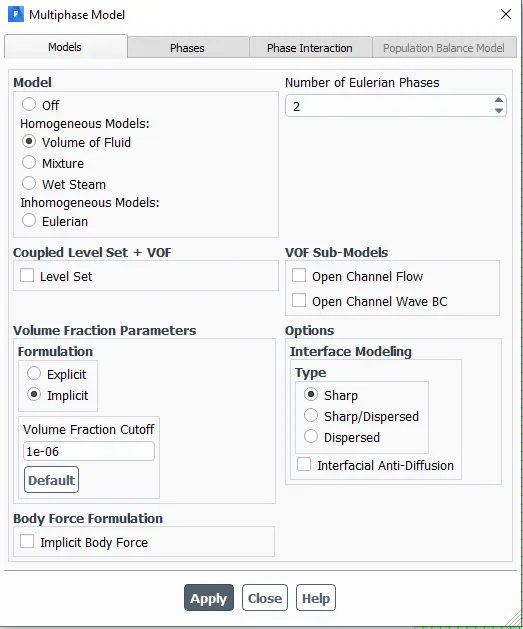
Here I choose VOLUME OF FLUID Method, as it is suitable for for COMPUTATIONAL simulations for tracking the volume of fluids at each time step.

MATERIALS:

After initialization surfaces were patched.

Calculation:

Timestep size: 0.005s

No. of Timesteps: 1000

Scaled Residuals for 0.5mm Mesh

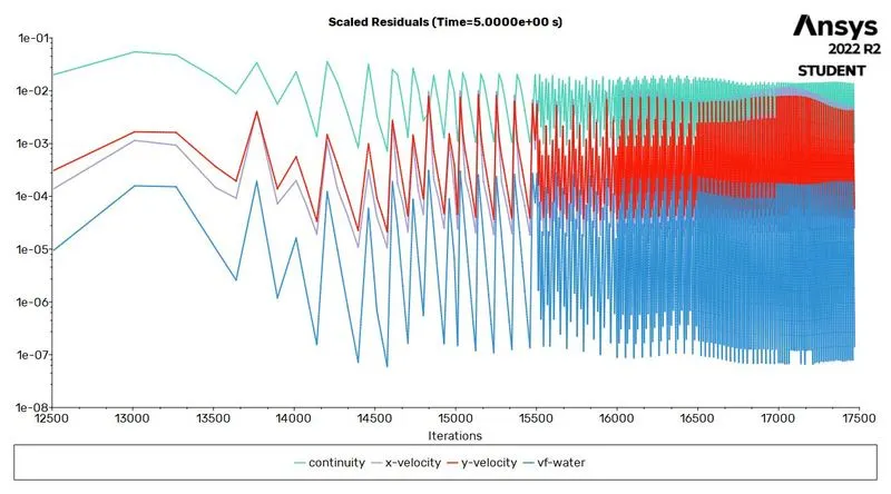
The residual plot is a graph that shows the convergence of a numerical simulation over time. In the case of a fluid instability simulation, the residual plot can be used to assess the accuracy and stability of the solution.

If the residual plot shows that the values are not much varied and the system came into a convergence state in a very small number of iterations and flow time, it indicates that the simulation is stable and has produced accurate results. This suggests that the numerical methods and solver used in the simulation are effective at capturing the dynamics of the fluid instability.

Volume Fraction Contour Plot

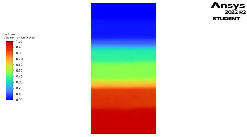
GIF File of MIXING PHENOMENON:

RESULT:

In the fluid instability simulation that was set up, the higher density fluid was placed above the lower density fluid, due to the effects of gravity. As the simulation progressed, the higher density fluid moved downwards while the lower density fluid moved upwards. This is a characteristic of the Rayleigh-Taylor instability, which occurs when fluids of different densities interact under the influence of an external force, such as gravity.

In the simulation, the inversion of the fluids from top to bottom was observed in the form of fingers. These fingers are a common feature of the Rayleigh-Taylor instability and are caused by the mixing of the two fluids at the interface. The simulation was run for a flow time of 5 seconds, and the resulting flow was observed to be a density stratified flow. This means that the fluids remained largely separate and did not mix significantly over the course of the simulation.

CASE 2:

In this case for the same geometry mesh size is changed for 0.1mm and also properties of water has been changed viscosity of water to 0.005kg/m-s. Remaining procedure followed is same. Below are the results.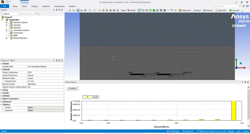

Mesh size =0.1mm

Mesh Element =Quad

Number of Elements=80000.

Quality of the mesh elements found satisfactory.

Scaled Residuals for 0.1mm Mesh

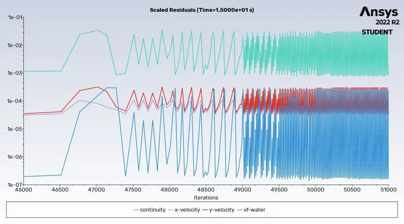
If the scaled residual results for a fluid instability simulation show that it took a longer time and a larger number of iterations to reach a state where there are not large fluctuations in the results, it may be due to the presence of a more viscous fluid in the simulation. The higher viscosity of the fluid can affect the stability and accuracy of the simulation by slowing down the flow and causing the residuals to converge more slowly.

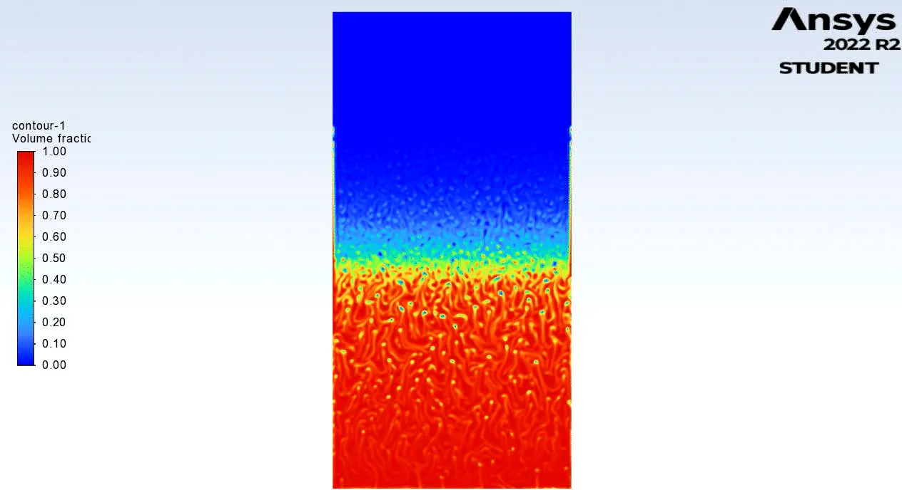
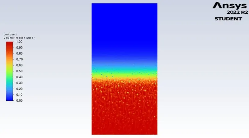
Volume Of Fluid :

RESULTS:

In the second case of the fluid instability simulation, the viscosity of the water was increased to 0.005kg/m-s. This made the water more viscous compared to the air, which was the other fluid in the interface. As a result, the water tended to stick to the walls and had a larger flow compared to the case where the viscosity was not changed.

As the simulation progressed, the higher density fluid (water) moved downwards first, and the lower density fluid (air) was trapped and moved upwards slowly in the form of bubbles. At the interface, the mixture of the two fluids appeared to be foam- or froth-like. This behavior illustrates the dynamics and instability of two different fluids when they interact at an interface. The relative viscosities of the fluids, as well as the external forces acting on them, play a significant role in determining the behavior of the fluids at the interface.

CONCLUSION:

In conclusion, the fluid instability simulation demonstrated how two fluids of different densities can behave when they interact at an interface under the influence of an external force, such as gravity. In the first case, the higher density fluid moved downwards while the lower density fluid moved upwards, resulting in the formation of fingers at the interface. In the second case, the viscosity of the water was increased, causing it to stick to the walls and flow more slowly compared to the air. As a result, the air was trapped and moved upwards slowly in the form of bubbles, while the water moved downwards.

Overall, the simulation showed that the relative densities, viscosities, and external forces acting on the fluids can significantly affect their behavior at the interface. Understanding these dynamics is important for predicting and controlling the behavior of fluids in various applications, such as rocket propulsion, volcanic fumes dispersion, and fluid flow in petroleum industry.