Week 5 - Rayleigh Taylor Instability

Aim - Perform the Rayleigh Taylor instability simulation.

Introduction - The Rayleigh–Taylor instability, or RT instability, is an instability of an interface between two fluids of different densities which occurs when the lighter fluid is pushing the heavier fluid.

This situation has engineering implications in several industries. For example, in die casting, liquid metal is injected in a cavity filled with air. In poor designs or other situations, some air is not evacuated and stay in small cavity on the edges of the shape to be casted. Thus, it can create a situation where the liquid metal is above the air but cannot penetrate into the cavity because of instability.

The Richtmyer–Meshkov instability occurs when there is an impulsive acceleration between two fluids. This type of instability can occur when there is a shock at greater speeds. The development of the instability begins with small amplitude perturbations which initially grow linearly with time. This is followed by a nonlinear regime with bubbles appearing in the case of a light fluid penetrating a heavy fluid.

The Plateau–Rayleigh instability, often just called the Rayleigh instability, explains why and how a falling stream of fluid breaks up into smaller packets with the same volume but less surface area. It is related to the Ryleigh- Taylor instability. and is part of a greater branch of fluid dynamics concerned with fluid thread breakup. This fluid instability is exploited in the design of a particular type of ink jet technology.

The Kelvin–Helmholtz instability (after Lord Kelvin and Hermann von Helmholtz) can occur when there is velocity shear in a single continuous fluid, or where there is a velocity difference across the interface between two fluids. An example is wind blowing over water: The instability manifests in waves on the water surface. More generally, clouds, the ocean, Saturn's bands, Jupiter's Red Spot, and the sun's corona show this instability.

Procedure- starting with the setting up geometry on the space claim till the getting final result is shown in the following steps.

Step_1 setting up the geometry on the space claim.

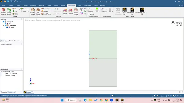
• Create the rectangle of 20*20 and name it as the air domain.
• Now again create the rectangle above this rectangle of same dimension and name it as the fluid domain.
• Use pull commend to convert the geometry into surface.
• Now use share topology between both the domain to share the mesh information, between both.

Step_2 mesh the geometry.

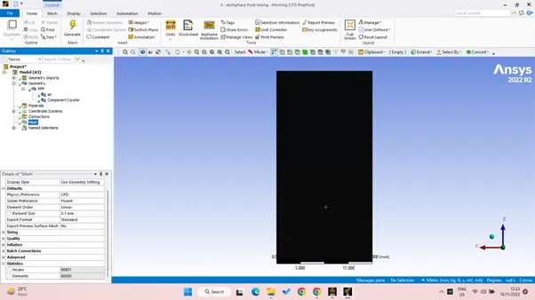
• As given in the question here we need to use the two separate mesh size and need to create two different result for the same.
• Thus first mesh size is 0.5mm.
• And second mesh size is 0.1mm, which is provided to the body sizing.
• Generate the mesh.
• Give the name selection as the upper domain has to be the denser fluid as to follow the Rayleigh–Taylor instability.
• Name Upper body as water and the lower body as the air.

Step_3 setting up the physics and solver.

• The solver that we setting up for the following geometry has to be the pressure base > transient with the gravity option enabled.
• Set the gravitational acceleration as in –y is 9.81m/s^2.
• The viscous model is to be the laminar model, as here we are not giving any inlet velocity to the fluid.
• Multiphase- In fluid mechanics, multiphase flow is the simultaneous flow of materials with two or more thermodynamic phases. Virtually all processing technologies from cavitating pumps and turbines to paper-making and the construction of plastics involve some form of multiphase flow.
• Volume of fluid method- In computational fluid dynamics, the volume of fluid (VOF) method is a free-surface modelling technique, i.e. a numerical technique for tracking and locating the free surface (or fluid–fluid interface).
• The multiphase solution should me implicit solution and assign the number of phase as 2.
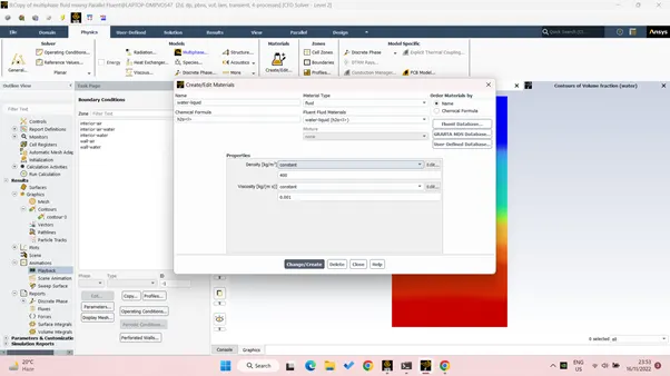
• Material as in the fluid air is already there we need to add the water from library.
• Also the phase-1 as air and phase-2 as water has been assigned.
• Hybrid initialise the solution.
• Now patch the volume as the phase value 1 to the water and 0 to the air.
• Here as mentioned in the question the another fluid is also taken with the specified material properties.

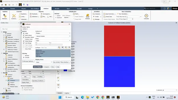
• Set the contour < filled < all body selected to see the animation.
• Also the create solution< under the animation < contour_1is selected, so the further animation can be saved as in the video form.

Result- the solution is stared with the time step size as 0.02 with the number of steps as 1000 to see the full result.

The result animation as in the video format is uploaded on the google drive and the link is attached here.

• For mesh size as 0.m

https://drive.google.com/file/d/1Gqqs544MiW9VYd2C3dmFEoEffVckxSfh/view?usp=sharing

• For mesh size as 0.5mm and with the new material having different properties.
  • density = 400 kg/m³,
  • viscosity = 0.001 kg/m-s

https://drive.google.com/file/d/1DXp_y8orKXK2Omv4uDhrnmwJ-SN1WU5z/view?usp=sharing

• for mesh size having 0.1 mm.

https://drive.google.com/file/d/1G_tFnz9Ktf_ILAgzfIw7V0RNzKxEwr6E/view?usp=sharing

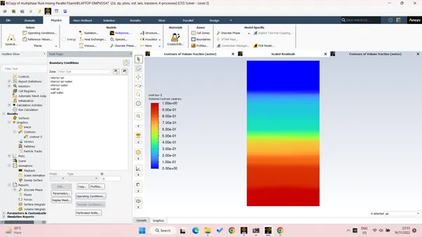
This image shows the animation over the contour after the solution is completed.

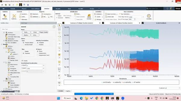
The residual plot here shows the solution is almost reached to the convergence.

Learning outcome - The Atwood number plays a critical role in describing the physics of fluids behind the hydrodynamic instabilities in fluid dynamics.

The results demonstrate that the Atwood number has a significant influence on flow morphology with wave patterns, vortex creation, vorticity generation, and bubble deformation.

For At > 0, the speed of the shock wave traveling along with the bubble inner surface is often less than that of the incident shock wave and greater than that of the transmitted shock wave.

For At ≈ 0, the incident and transmitted shock waves move at the same speeds.

for At < 0, the transmitted shock wave travels faster than the incident shock wave.

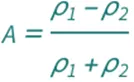
symbol	description	physical quantity
A	Atwood number	"Atwood Number"
ρ1	fluid density	"Mass Density"
ρ2	fluid density of lighter fluid	"Mass Density"

The Atwood number for the

• air and water having densities.

Water - 997 kg/m³

Air- 1.204 kg/m³

A = 0.9975

• air and the given material

Water - 997 kg/m³

Air- 400 kg/m³

A = 0.4273

Conclusion – This challenge was very different here, where instead of generating the solution and then analysis it with given data, I have to first learn the theories related to the challenge which is the Rayleigh –Taylor instability and then generating the real world simulation by the use of ANSYS fluent where physic was settled up so all the governing equation can be utilised in generating the data.

This challenge helped me in learning the new theory concept and also how there fundamental fluid concept can be simulated by using ANSYS Fluent so the real world problem can be solved.