Week 1- Mixing Tee

Aim - Introduction to GUI based CFD using ANSYS Fluent – Challenges Week 1- Mixing Tee.

Introduction – Mixing tee is the kind of device where two fluid having different velocity and temperature comes from two valve which is separated in 90 degrees and mixed inside the model, after mixing of the flued what changes occur in the properties of the fluid like temperature. Velocity, and pressure.

By the use of ANSYS fluent we can see the mathematical change in the fluid velocity in the visual forms with meshing and the colour combination.

Procedure and modelling approach (with the solver setting)- our modelling approach for the mixing tee model starts with the following steps.

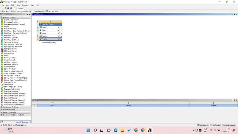
step -1 where we set our geometry for the modelling. Here we are using the already provided model with the challenge which is 0.9 m in length (approx.). for the given geometry under the ANSYS fluent we will open the space clan where our first step is the volume extraction. Prepare<volume extraction< select edge<finish< hide the geometry< supress for the physics. Close the window it will automatically save the model for the upstream step.

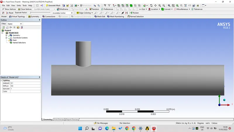
Step-2 Here in the second step our task is to performed the mesh generation over the model, for that we will set the appropriate mesh element size for the more refined structure.

But before we will give some appropriate name to all the face of our geometry. Select face< name< inlet-x< inlet-y< outlet< and the wall. Generally, the inlet –y is for the cold fluid and inlet x is for the hot fluid.

Now after providing the element size we will generate the mesh over the model.

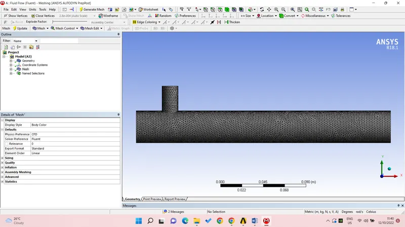
Step-3 in the 3rd step we will open our geometry in the fluent setup, where our task is to setup the equation and the boundary condition for the model.

Setting up the physics<steady< enable pressure option<energy option<absolute velocity<viscosity<k-epsilon (Reynold average naiver stroke model) <realization<ok

The material is air (idol gas), for the boundary condition < zones< cell zone<volume< edit for inlet-x the velocity is 3 m/s (given) and the temperature is 292.5k and for the inlet-y 6m/s (momentum ratio-2) and the hot temperature 309.15k (36 degrees Celsius) outlet will have zero given value.

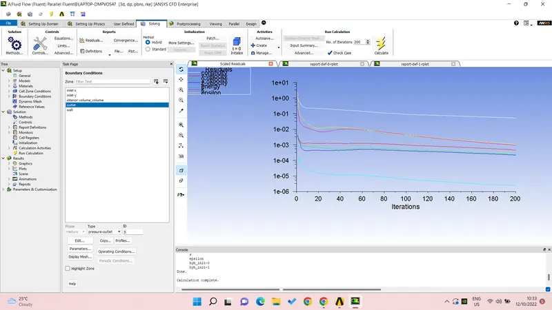
Under solving will define the mixing properties for the report generation with the temperature values in the y axis with area weightage and standard deviation with report file and report plot under 1 iteration,

Again in the solving method< hybrid initialization<and the given values for the iteration is 250 and generate will give us the plot.

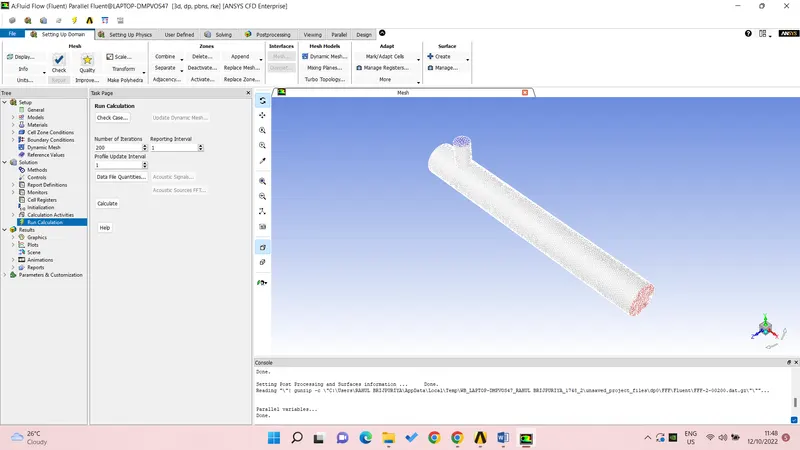
For the momentum ratio-4 the generate graph is

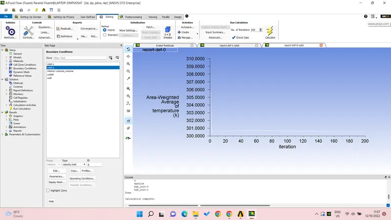
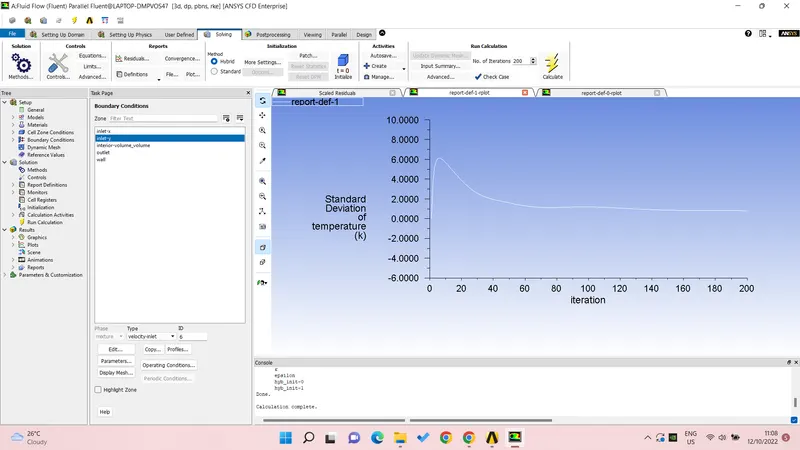
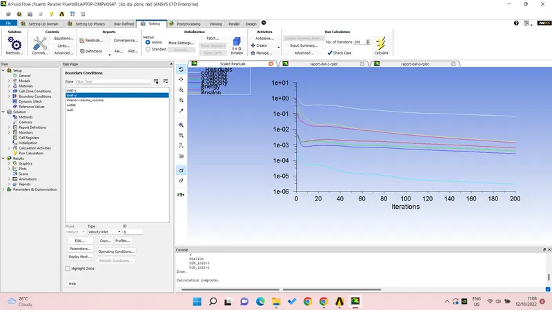
And for the momentum ratio is 2 the generated graph is-

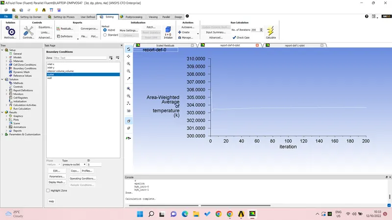
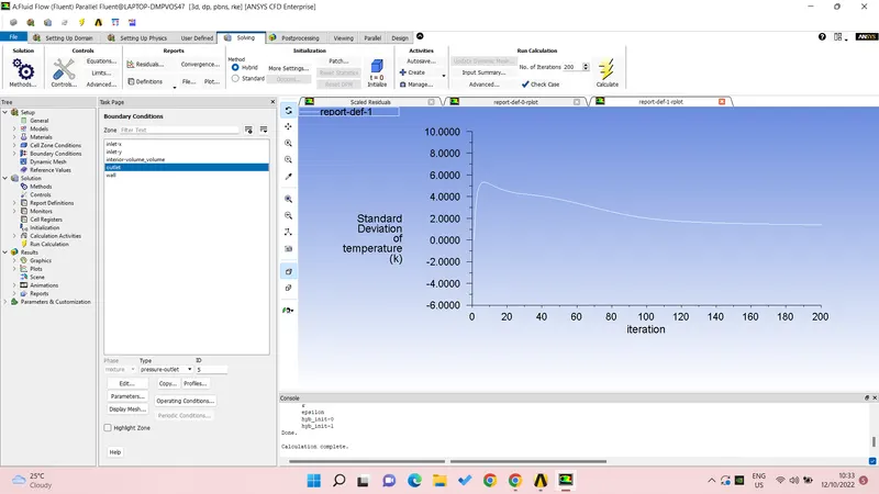
Step-4 – in the last step we will see our result but for this we have to insert the plane in our geometry with z=0 and in the xy plane with the less wall transparency so we can see the result on the plane also provide the white colour to the plane.

Plane<colour<variable<temperature<appetence<temperature<user define< the low and high limit of the temperature< apply we can see our result in the plane with some colures with fluid mixing.

The colour setting is for the legend view<fixed< two decimal place.

We can also see the generated mesh lines in our plane with show mesh lines.

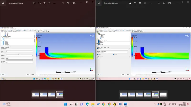
This is the refined result with the small mesh element size and appropriate given properties value.

For the momentum ratio-2

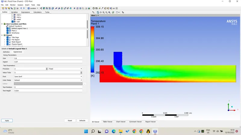
And for the momentum ratio-4

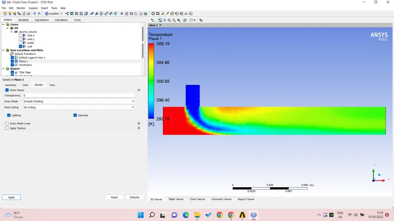
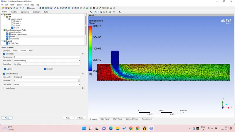
Result- here we can see the comparison in the both the result as the inlet velocity is just double in the second

(right side) case the outlet temperature is more on green colour which is around 300.15k.

Type of pipe(length)	Inlet velocity (m/s)		Mesh element size	No of iteration	Average outlet temperature (k)
	Hot	cold
Long pipe	3	6	2e-3	250	302-304
Long pipe	3	12	2e-3	250	300.15

And in the first image with the 6m/s cold inlet we have the mixed colour combination of red and green.

Conclusion- the ANSYS is the very vast software and here we have used fluent option for our fundamental calculation of mixing fluid with the different inlet condition to see the end result in the outlet.

As we can see in the difference in the result with the size of the model and the inlet condition, so to learn the software we have to do the lots of changes in the inlet condition to see the changes in the outlet it will make us the more grasp over the software tool.

I have faced few challenges while doing the mesh as to open the solid works file in the space clan to the installation of the software and for the more refine result providing the more refine mesh element size, but as in the end the challenges ended up with the new learning and the confidence.