Week 5 - Rayleigh Taylor Instability

Rayleigh Taylor Instability

Aim :- To perform the Rayleigh Taylor instability simulation for 2 different mesh sizes with the base mesh being 0.5mm.To explain the results by showing the animations and to study the effect of mesh size on simulation. We use Water and Air in this simulation and in one more case we use Water and a User-defined material having density = 400kg/m^3 and viscosity = 0.001kg/m-s . In these simulayions we have to suspend Water over Air and User-defined material and then we have to run the simulations and make an animation by calculating the Water Volume fraction.

Introduction and Theory :-

Rayleigh Taylor Instability :- The Rayleigh Taylor instability or RT instability (named after Lord Rayleigh and G.I Taylor), is an instability of an interface between two fluids of different densities which occurs when the lighter fluid is pushing the heavier fluid. Examples include the behaviour of water suspended above oil in the gravity of earth, mushroom clouds like those from volcanic eruptions and atmospheric nuclear explosions,supernova explosions in which expanding core gas is accelerated into denser shell gas,instabilities in plasma fusion reactors and inertial confinement fusion.

• Water suspended atop oil is an everyday example of Rayleigh-Taylor instability,and it may be modelled by two completely plane-parallel layers of immiscible fluid,the denser fluid on top of the less denser one and both subjecting to the Earth's gravity.This was the set-up as studied by Lord Rayleigh.If a parcel of heavier fluid is displaced downward with an equal volume of lighter fluid displaced upwards, the potential energy of the configuration is lower than the initial state.Thus the disturbance will grow as the denser material moves down under the gravitaional field. As the RT instability develops, the initial peturbations progress from a linear growth phase to a non-linear growth phase,eventually developing "plumes" flowing upwards (in the gravitational buyoyancy sense) and "spikes" falling downwards.
• The evolution of the Rayleigh Taylor instability involves 4 main stages.In the first stage the perturbation amplitudes are small when compared to their wavelengths,the equations of motion can be linearized,resulting in exponential instability growth.At the end of his first stage,when non-linear effects begin to appear,one observes the beginnings of the formation of the mushroom shaped spikes.The growth of the mushroom structures continues in the second stage and can be modeled using buoyancy drag models.The spikes and bubbles then begin to interact with one another in the third stage.Bubble merging takes place,where spikes and bubbles of smaller wavelength that have become saturated are enveloped by larger ones that have not yet saturated.This eventually develops into a region of turbulent mixing,which is the fourth and the final stage in the evolution.

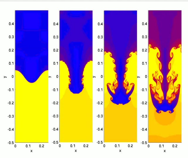
Crab Nebula:-

Some practical CFD models that have been based on the mathematical analysis of Rayleigh Taylor waves :-

Kelvin-Helmholtz instability (named after Lord Kelvin and Hermann von Helmholtz):- The Kelvin-Helmholtz instability can occur when there is a velocity shear in a single continuous fluid,or where there is a velocity difference across the interface between two fluids.An example is 'Wind blowing over Water' The instability manifests in the waves on the water surface.The theory predicts the onset of instability and transition to turbulent flow in fluids of different densities moving at various speeds. Helmholtz studied the dynamics of two fluids of different densities when a small disturbance such as a wave,was introduced at the boundary connecting the fluids.For a continuously varying distribution of densities and velocities (with the lighter layers uppermost, so that the fluid is RT-stable) the dynamics of the KH instability is described by the Taylor-Goldstein equation and its onset is given by the Richardson number (Ri)

Plateau Rayleigh Instability :- The Plateau Rayleigh instability explains why and how a falling stream of fluid breaks up into smaller packets with the same volume but less surface area.It is related to the Rayleigh Taylor instability and is a part of a greater branch of fluid dynamics concerned with the fluid thread breakup.This fluid instability is exploted in the design of a particular type of ink jet technology where a jet of liquid is perturbed into a steady stream of droplets. The driving force of the Plateau Rayleigh instability is that liquids, by virtue of their surface tensions , tend to minimize their surface area.

Buoyancy Drag model :- It is a model which uses ordinary differential equations to evolve the width of the mixing layer.These models can't model multiple mixing interfaces,also donot adress demixing known as counter gradient transport i.e, reduction of total fluid masses within the mixing zone.

K-L model :- The K-L model was proposed by Dimonte and Tipton for describing the turbulent self similar regime of RT and RM induced mixing.

Computational methodology :-

• All the simulations were performed with SIMPLE algorithm using 2nd-order Upwind scheme.To account for the difference in accuracy,the grid spacing is refined.
• The steady state analysis is used when we are more concerned with the end result.But for Rayleigh-Taylor instability we are more interested in observing the real time changes of the interface and the fluid region.The real time observation is possible in Transient state analysis.In steady state simulation we can't see the small time variation of instability and it is used for the final state results.

Performing the Rayleigh Taylor instability simulation for 2 different mesh sizes(with the base mesh 0.5mm) :

Geometry :- Click and drag Ansys Fluent in Ansys workbench to create a new project and name it Rayleigh Taylor instability.

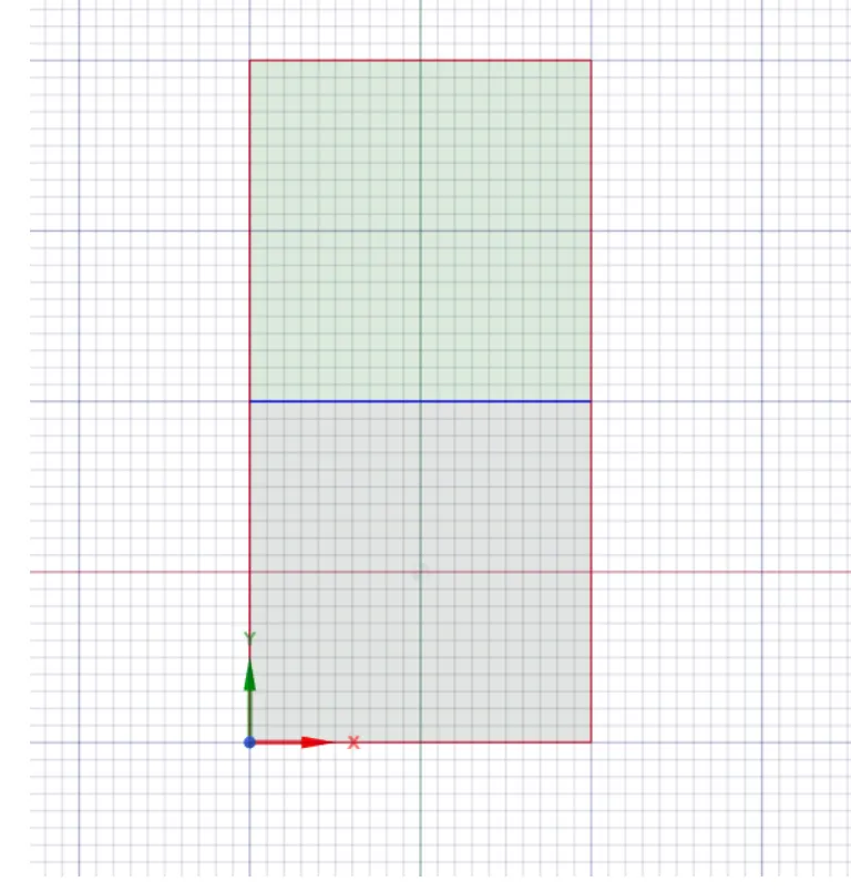
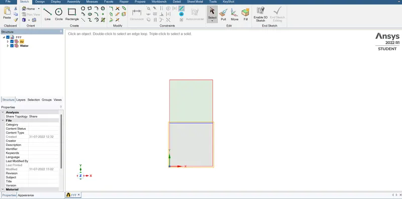
1. Double click on geometry to open the spaceclaim and now we have to create two squares of dimensions 20mm X 20mm one upper and the other lower.
2. First create the lower volume and then extract it,then create the upper volume and then extract it.
3. Name the lower volume as 'Air' and the upper volume as 'Water'.
4. And then share the topology such that they share one interface edge.(Use 'shareprep' tool from workbench.)
5. Now close the geometry.

Meshing :-

1.Open Meshing section and click on the element size and set it to 0.5mm.

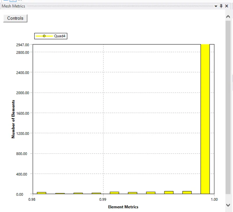
2.Now click on generate mesh and observe the meshing.(Nodes = 3321,Elements = 3200)

3.Check the number of nodes and elements and check the quality and then close the meshing.

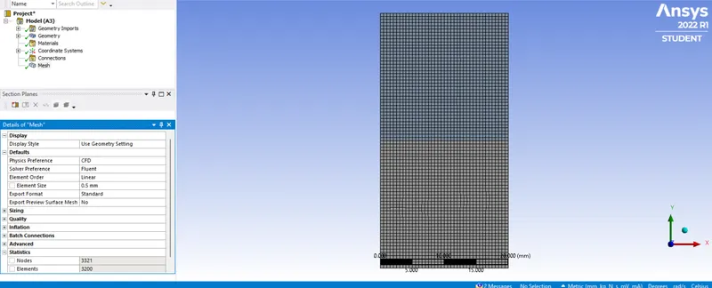
Element quality

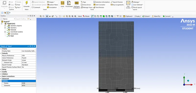
Refined Mesh - (Element size = 0.3mm) Nodes = 9180, Elements = 8978.

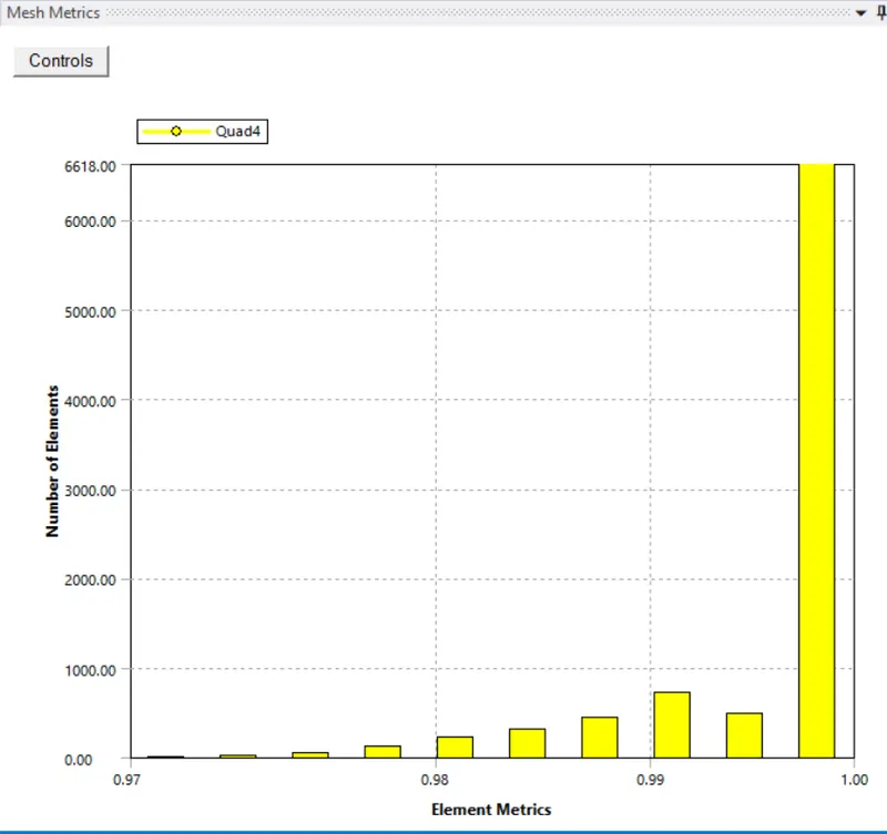
Element Quality

Setup :-

1.Select the pressure based solver and transient state approach.

2.Select gravity and give the values X = 0m/s^2 , Y = -9.81m/s^2.

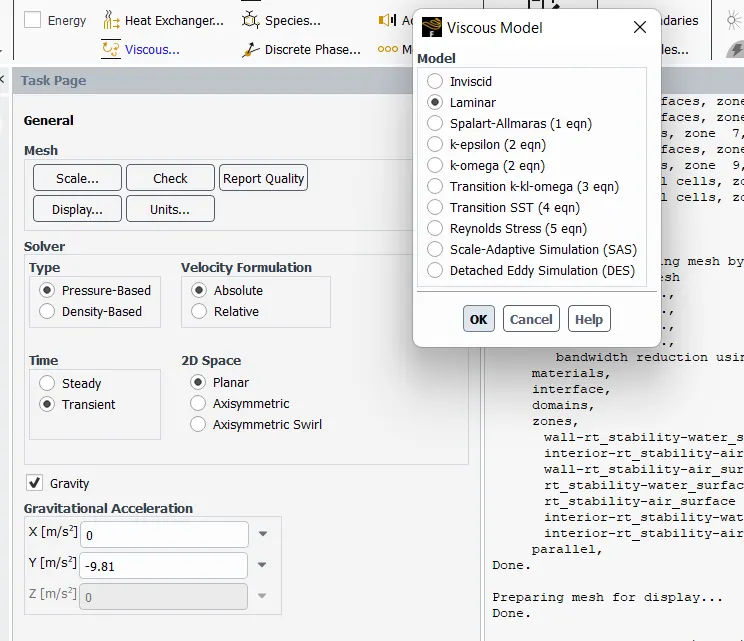
3.Select the viscous model and select Laminar model.

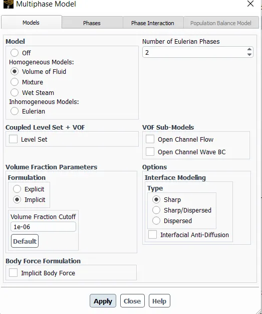
4.Go to multiphase model and select volume of Fluid model and then set implicit formulation.

5.Here Energy equation is not used since there is no temperature involvement.

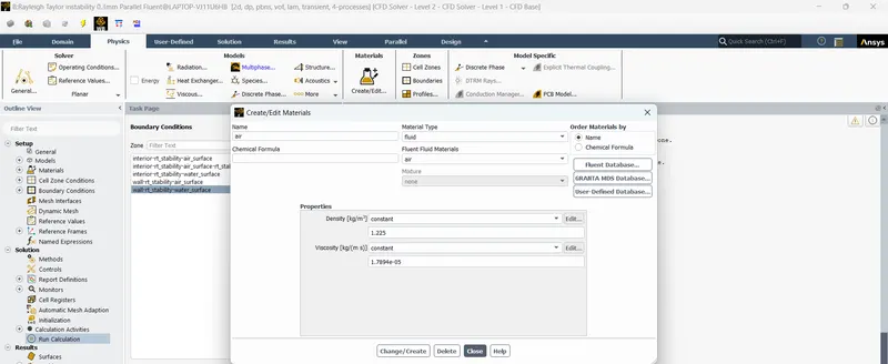
6.Now click on materials and add the materials , we are using 'air' and 'water' in this simulation.

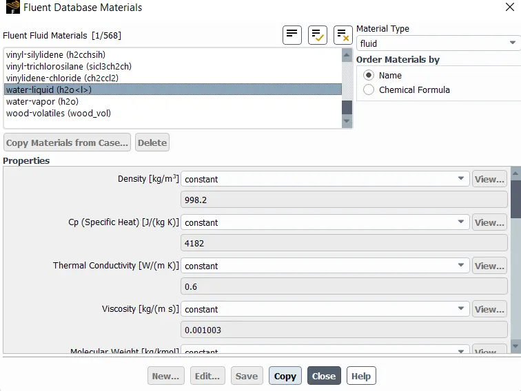
Add water from Fluent Database Materials

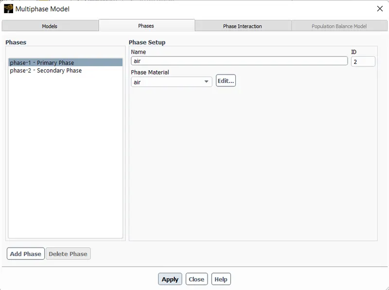
7.Now go to multiphase and click on phases,select 'air' as primary phase material and 'water' as secondary phase material.

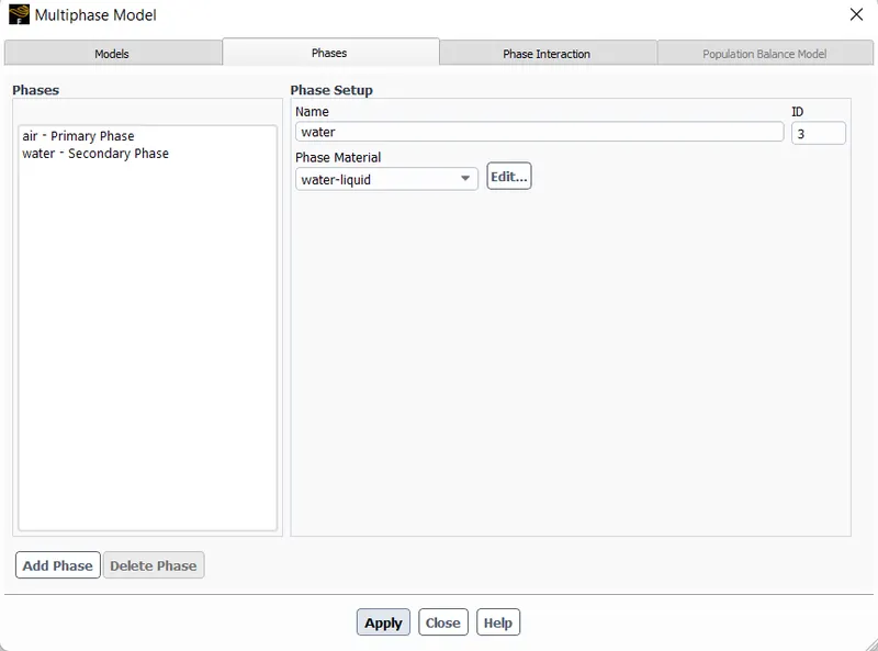
8. Check the domain and see that the bottom surface is 'air' and the upper surface is 'water' for confirmation.

9. Also perform mesh check

10. Initialize the problem with standard initialization method since we are using transient state approach.

11. In the third case of the simulation we have to give a user-defined material in Materials in place of 'air' and set it to Primary phase. Water is to be given as second phase material as usual.

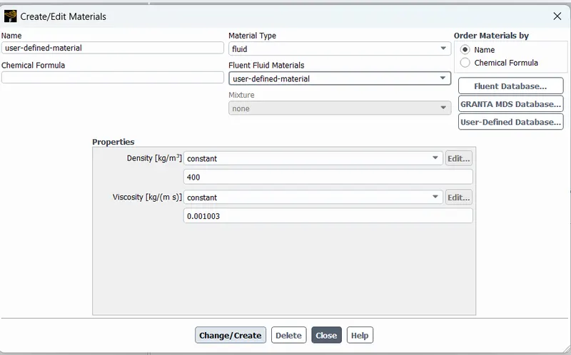
12. And now go to domain and check the zones and just display and see the surfaces to remember what we have to Patch. (i.e Ansys allocates various names to the surfaces and we have to remember the water surface)

13. Now select standard initialization method and click on " t=0 Initialize ".

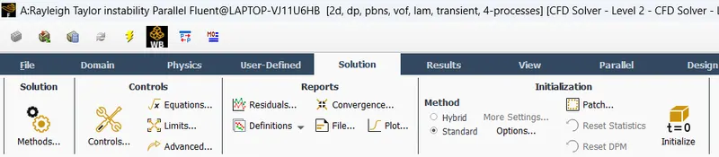
14. Now Go to Patch and for water set the Volume fraction = 1 for water surface (rt-stability_water-surface) and 0 for air surface

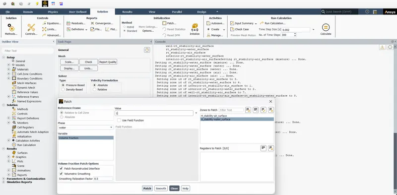
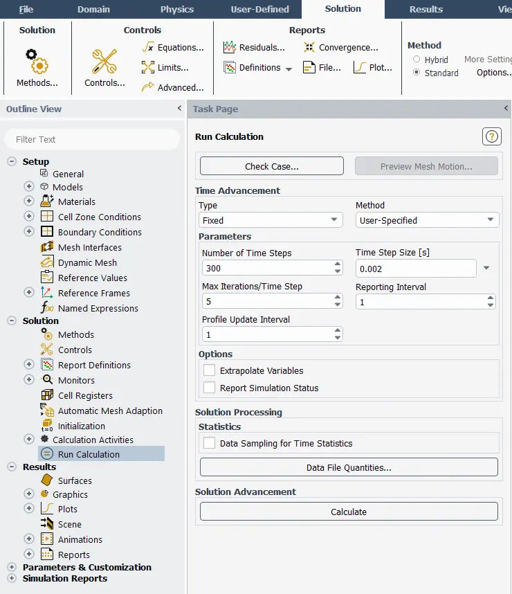
15. Now under solutions - calculation activities, double click on Run-calculation, select Fixed type,give the number of time steps = 300, Timestepsize = 0.002,

16.Create a Countour for Volume Fraction for water phase.

17.Create a Time step animaton for the Volume fraction of water for every two time steps.

18. Run the calculation.(Wait for sometime to complete the calculation by Ansys, if you find any floating point error then check the meshing again and check quality criteria, aspect ratio and give better element size and do meshing and again do the calculation. *Note - whenever you re-run the calculation you have to patch the volume fraction of water to 1)

Results :-

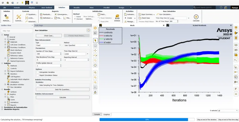
Scaled residuals

• Rayleigh Taylor Instability Animation video - 0.5mm grid (Water and Air)

• Rayleigh Taylor Instability Animation video - 0.3mm refined Grid (Water and Air)

• Rayleigh Taylor Instability Animation video - 0.3mm Grid (Water & User-defined-material)

Atwood number(A) :- It is a dimensionless number which is used to study hydrodynamic instabilities in density stratified flows.

A = (ρ1 - ρ2) / (ρ1 + ρ2) where ρ1 is density of heavier fluid and ρ2 is density of lighter fluid.

For Air & Water RT instability ρ1 = 998.2kg/m^3 and ρ2 = 1.225kg/m^3, A = 0.9975

For user-defined material & Water RT instability ρ1 = 998.2kg/m^3 and ρ2 = 400kg/m^3, A = 0.4278

Behaviour of the Atwood number on instability :-

Rayleigh Taylor Instability evolves in 3 distinct stages. Linear stability, Mushroom head falling or Bubble rise formation, long term evolution due to bubble merging and mixing. for low Atwood number, bubble and mushroom head shape is relatively symmetrical.The disturbances are linear for a larger time. For large Atwood number, bubble and mushroom shapes are less symmetrical and it occurs rapidly leading to a non-linear growth rate.

Conclusion :- The mesh with smaller element size gives the rayleigh taylor instability waves better than the mesh with larger element size. But it takes more time for the simulation to complete the calculation in case of finer mesh.

Compared to air, the user-defined material has more density and so it takes more time to settle down.

Since the simulation involves capturing instabilities which are changing in an unpredictable manner as a function of time, transient approach is preffered over steady state approach.So the steady state approach might not be suitable for these simulations.