Week 5 - Rayleigh Taylor Instability

Aim: 

• To study the concept of Rayleigh Taylor Instability and some practical CFD models that have been based on the mathematical analysis of Rayleigh Taylor waves.
• To study the Rayleigh Taylor Instability simulation for 2 different mesh sizes in addition to baseline and compare the results.
• To study the the effect of Atwood number variation on Rayleigh Taylor Instability for all the cases.

Given:

• Baseline mesh size= 0.5mm or 0.0005m
• Materials selection - Air, water and user-defined material(density = 400 kg/m3, viscosity = 0.001 kg/m-s)

Introduction:

Rayleigh Taylor Instability is an instability of the interface between the two fluids of different densities which occurs when the lighter fluid is pushing the heavier fluid. It is clear from Newtons law of viscosity; fluid cannot resist the slightest shear force and Density is one of the main property of the fluid to incorporate the shear force. Based on the density, when lighter and heavier fluids are mixed together, denser fluid comes to top of the lighter fluid, due to the gravity and the density variation at the interface of the liquid is not stable. This instability of the interface between the different densities of fluid when the lighter fluid is accelerated towards the heavier fluid is called RAYLEIGH TAYLOR INSTABILITY.

Examples:

• Formation of high luminosity twin exhaust jets in rotating gas clouds in an external gravitational potential,
• Instabilities in plasma fusion reactors and intertial confinement fusion,
• Electromagnetic implosion of metal liner
• Behaviour of water that is suspended above oil in gravity of Earth

What are some practical CFD models that have been based on the mathematical analysis of Rayleigh Taylor waves?

Practical CFD models:

SPH method(Smoother particle hydrodynamics)

Smoothed-particle hydrodynamics (SPH) is a computational method used for simulating the mechanics of continuum media, such as solid mechanics and fluid flows. Smoothed-particle hydrodynamics is being increasingly used to model fluid motion as well. This is due to several benefits over traditional grid-based techniques. First, SPH guarantees conservation of mass without extra computation since the particles themselves represent mass. Second, SPH computes pressure from weighted contributions of neighboring particles rather than by solving linear systems of equations. Finally, unlike grid-based techniques, which must track fluid boundaries, SPH creates a free surface for two-phase interacting fluids directly since the particles represent the denser fluid and space represents the lighter fluid.

SINGLE-FLUID MODEL:

A typical approach used for the analysis of two-phase flows is a mixture model, i.e. the individual fluid phases are assumed to behave as a flowing mixture described in terms of the mixture properties. The applied single-fluid model is a five-equation model consisting of the mass, momentum, and energy equations for a vapor/liquid mixture, and two equations describing the formation and growth of the liquid phase.

TWO-FLUID MODEL:

In the two-fluid model, separate sets of the governing equation for the vapor and liquid phases have been used. The interaction between the droplets and the heat exchange between the liquid phase and the solid boundary is not modeled here as well. Additionally, the velocity slip between the vapor and the liquid phase is in this model considered.

Turbulence model:

Turbulence models are needed to predict the average mixing behavior inflows that are on average one- or two-dimensional. The approach to the construction of the tile turbulence model is guided by experimental behavior. The equations governing turbulent flows can only be solved directly for simple cases of flow. For most real-life turbulent flows, CFD simulations use turbulent models to predict the evolution of turbulence. These turbulence models are simplified constitutive equations that predict the statistical evolution of turbulent flows

Geometry preparation:

• OPEN IN SPACE CLAIM
• Create a square of 20mm*20mm.Use Pull tool in order to create a surface.
• Move the generated component to the New Component. Name it as Air. Now click on design and create a new component --> Water. Repeat sketch just above the Air with the similar dimensions as mentioned.
• Check if both the components i.e Air and Water are created.
• Workbench > click on Share > Ok

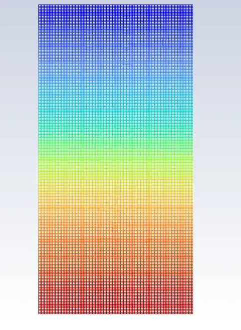
CASE 1: element size 0.5mm

Mesh:

OPEN MESH --> Generate the mesh --> baseline mesh 0.5mm

Set Up:

• SETTING UP DOMAIN -->MESH --> select CHECK. Then in CONSOLE WINDOW --> it shows 'CHECKING MESH…. DONE' 
• SETTING UP PHYSICS --> SOLVER --> select Time = Transient, Type = PRESSURE BASED & Velocity Formation = ABSOLUTE, enable gravity in y- direction (-9.81)
• VISCOUS MODEL --> Laminar--> OK. 
• Material selection. Materials -->Air and Water.
• Multiphase--> Model=Volume of Fluid, select Implicit Formulation, -->Number of Eulerian Process is 2. 
• Phases --> primary phase=Air(phase-1) and secondary phase=Water(phase-2).
• Solving -->Method=standard --> Patch--> Phase=Water, Variable=Volume Fraction --> select water_surface=1 --> click Patch. Similarly for air_surface=0 --> click Patch.
• α= 1 means fluid on top, and αα= 0 means fluid is below
• To check initialization is done properly or not, go to postprocessing
• Postprocessing --> create contours --> contour of= Phases, Phase=water, select all the surfaces --> Save/Display. Now contour is generated showing water at top and air at bottom.
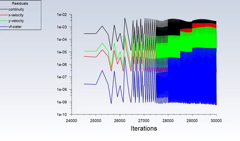
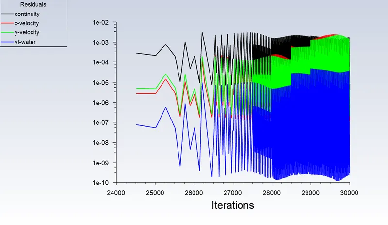
• Run-->Calculation > Type=Fixed Time Step, Time step Size=0.005, Number of iterations=1500 --> click Calculate.
• create solution animation for above contour to check the simulation 

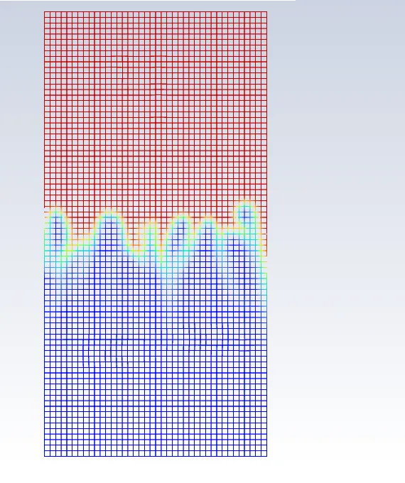
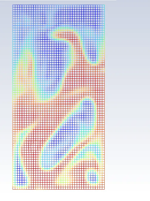
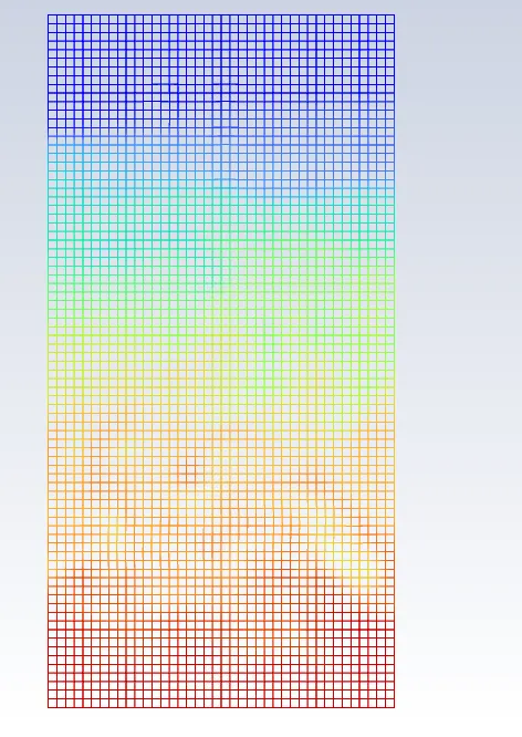
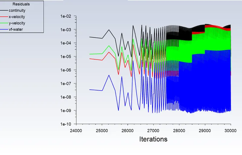
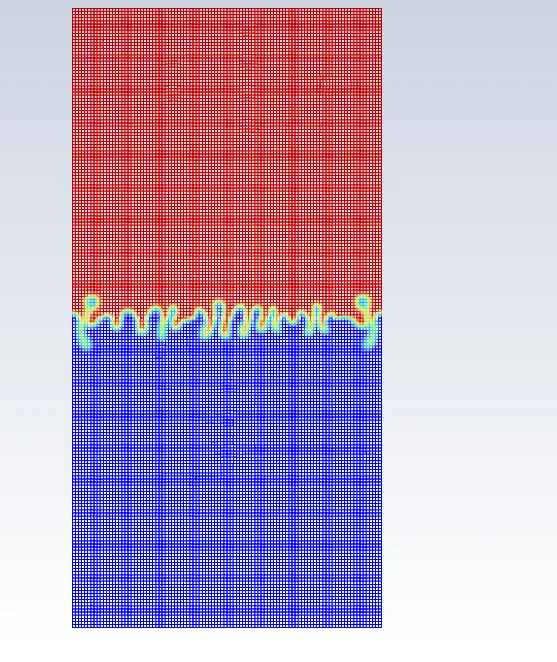
CASE2: element size 0.2mm

Follow the above procedure

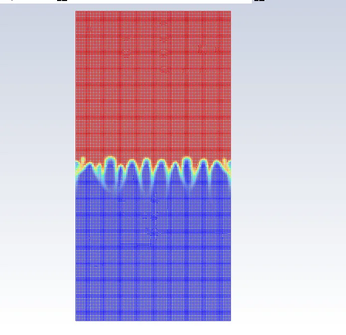
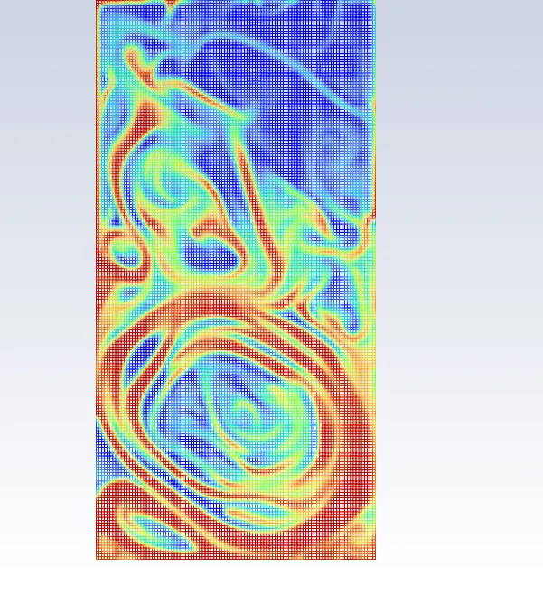
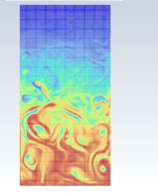
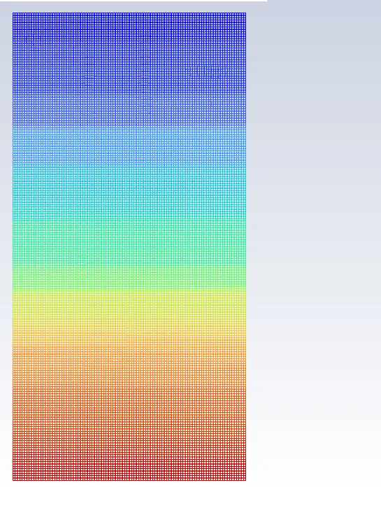
CASE3: element size 0.2mm

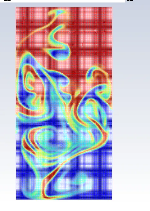
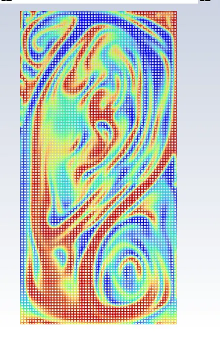
material: phase1 – user defined material

               phase2 - water

Atwood Number:

It is a dimensionless number in fluid dynamics used in the study of hydrodynamic instabilities in density stratified flows. It is a dimensionless density ratio defined as:

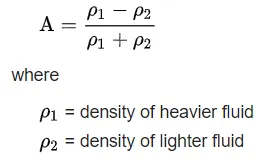
• It is paramount in the study of Rayleigh-Taylor instability. 
• Atwood number close to 0, RT instability flows take the form asymmetric “finger” of fluid; 
• Atwood number close to 1, the much lighter fluid “below” the heavier fluid takes the form of larger bubble-like plumes.

The behaviour of RT Instability on the variation of Atwood number:

RTI evolves in three distinct stages: Linear stability, mushroom head(falling) or bubble(rising) formation, long term evolution due to bubble merging and mixing. For low Atwood number, bubble and mushroom head shape is relatively symmetrical, the disturbances or perturbations are linear for a larger time. In contrast, for large Atwood number, bubble and mushroom head shape is less symmetrical, also it occurs very rapidly at an accelerating rate which leads to a nonlinear growth rate.

CONCLUSION:

• Rayleigh Taylor Instability simulation was studied at interface of both fluids having different densities under the influence of gravity and the following observations were made:
• From the above cases, we observe that finer mesh captures the instability better than the coarse mesh, but it takes more time for the heavier fluid to settle down. As computational time is long but produces results with better accuracy.
• Since the simulation involves capturing instabilities that are changing in an unpredictable manner as a function of time, the transient approach is preferred over the steady-state approach. 
• The Atwood no validates the CFD simulation as it is observed. In the case of water and air mixing, bubble formation takes place, whereas in the other case no bubble takes place.
• The Atwood number depends on the density of the fluid and ranges from 0 to 1.
• Both cases have larger Atwood number showing the Rayleigh Taylor Instability.