Week 5 - Rayleigh Taylor Instability

1. What are some practical CFD models that have been based on the mathematical analysis of Rayleigh Taylor waves? In your own words, explain how these mathematical models have been adapted for CFD calculations.
2. Perform the Rayleigh Taylor instability simulation for 2 different mesh sizes with the base mesh being 0.5 mm. Compare the results by showing the animations( Attach them from your google drive). Observe the differences in the animation and explain the effect of mesh size on simulation. Also, explain why a steady-state approach might not be suitable for these types of simulation.[ Choose Air and Water for this simulation]
3. Run one more simulation with water and user-defined material(density = 400 kg/m³, viscosity = 0.001 kg/m-s) for refined mesh.
4. Define the Atwood Number. Find out the Atwood number for both the cases and explain how the variation in Atwood number in the above two cases affects the behavior of the instability.

AIM:

To perform the Rayleigh Taylor instability simulation by using ANSYS FLUENT for the given cases.

OBJECTIVE:

• To perform the Rayleigh Taylor instability simulation with water and air as the fluids in first part and with water and a user defined fluid with density = 400 kg/m³, viscosity = 0.001 kg/m-s in the second part.
• Perform the simulation by using basline and fine meshing for part 1 and compare the results.
• To define Atwood number and to calculate the same for the given cases.

THEORY:

Rayleigh Taylor instability is the instability of interface between two fluids of different densities ocuurs due when the lighter fluid is pushing the heavier fluid. Example of RT instability is the behavior of water suspended above oil in the gravity of Earth.

Practical CFD models that have been based on mathematical analysis of RT waves.

• Kelvin-Helmholtz instability
• Richtmyer-Meshkov instability
• Plateau-Rayleigh instability

Kelvin-Helmholtz instability mainly occurs when there is a velocity difference across the interface of two fluids. Example of such instabilites can be observed when wind blows across a water surface.

Richtmyer-Meshkov instability mainly occurs when two fluids with different densities are accelerated suddenly. Mainly this happens due to passage of a shock wave through the fluids. The instability begins with small amplitude perturbations which initially grow linearly with time and followed by a nonlinear regime.

Plateau-Rayleigh instability is called as Rayleigh Instability which explains how a falling strean of fluid breaks into smaller packets with same volume but less surface area. The main driving force of this instability is the surface tension which tend to minimize the surface area.

PROCEDURE:

GEOMETRY

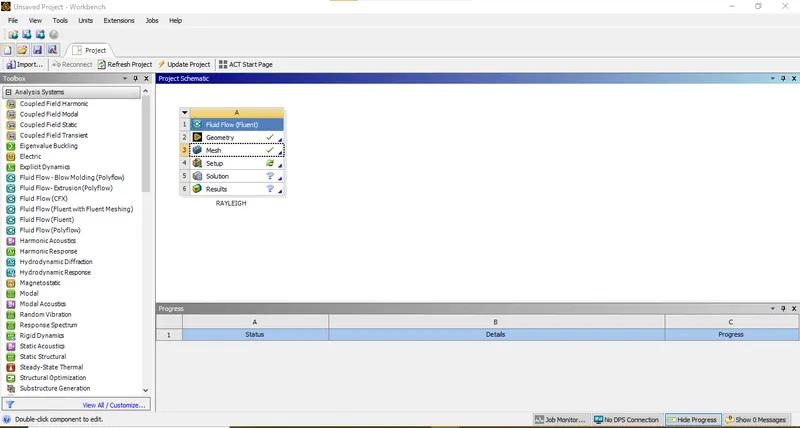
• Open ANSYS Workbench 2022R2 select Fluid Flow (Fluent) from Toolbox.

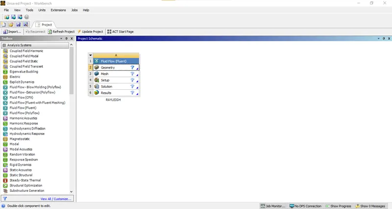
• Rename the file and left click Geometry and select New Spaceclaim Geometry.

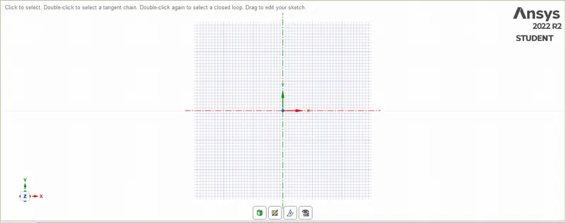
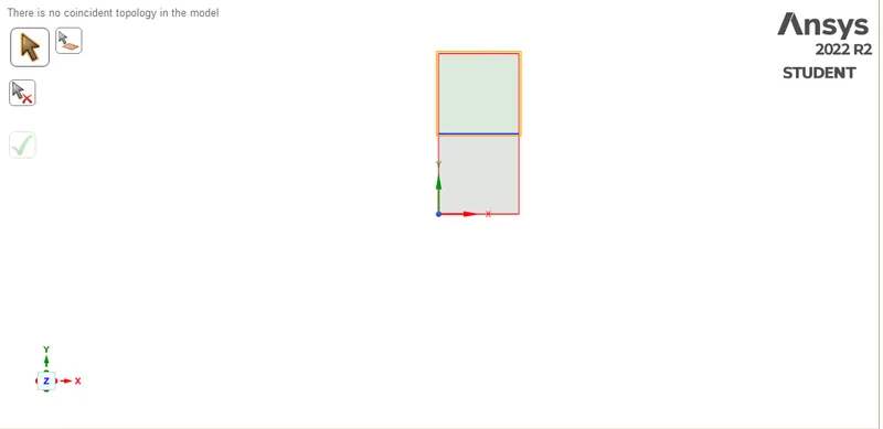
• Create the geometry as shown below using rectangle tool and create surface by using Fill option and rename the surfaces as solid and fluid. The created geometry is shown in the below figure.

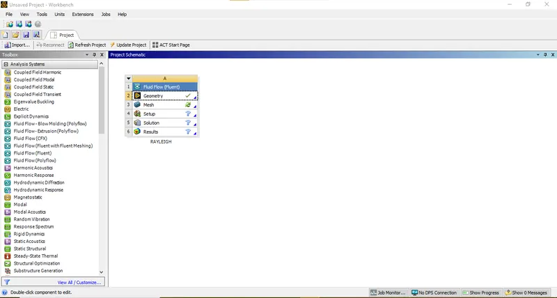
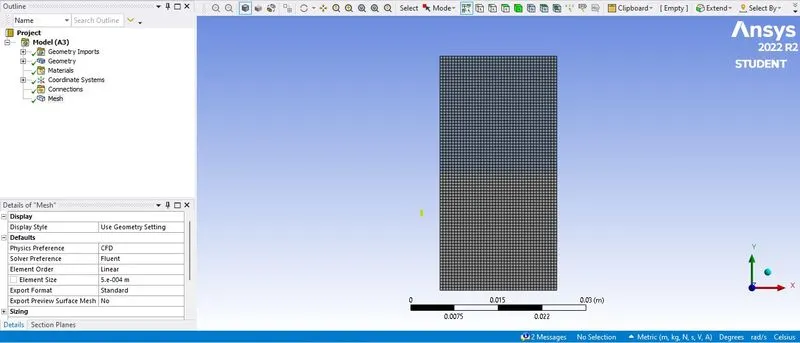
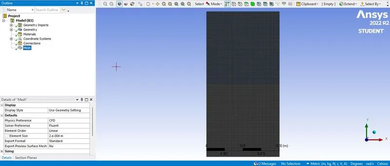
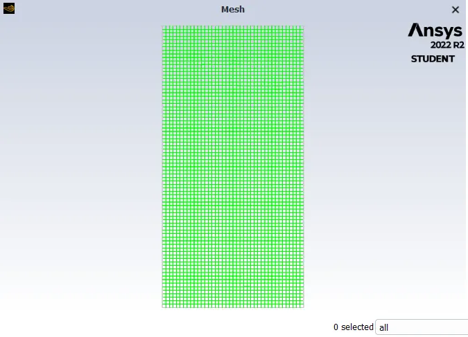
• Close SpaceClaim and double click on Mesh. Meshing window will appear. Now select the mesh from the tree and generate mesh with an appropriate element size of 50 mm for baseline meshing and 20mm for fine meshing. Perform the second part of the question (Water and user defined fluid) by using the fine meshing. The figures shown below are the final meshed geometry for both the cases.

MESH

Baseline meshing (element size = 50mm)

Fine meshing (element size = 20mm)

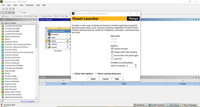
• Close Meshing and double click on Setup, select Double Precision and Fluent window will open. Check all the values and make necessary correction if needed.
• Select the conditions mentioned below.

SETUP

SIMULATION SETUP DETAILS:

I. SETUP PHYSICS

SOLVER

Typer --> pressure based

velocity Formulation --> Absolute

Time --> Transient

2D space --> planar

Gravity - Tick the check box

Gravitational Acceleration

X (m/s2) = 0

Y (m/s2) = -9.81

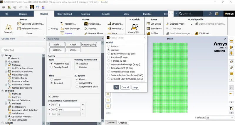
MODELS

Viscous --> Laminar

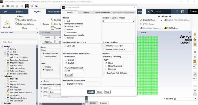
Multiphase

Model --> volume of Fluid

Formulation --> Implicit

MATERIALS

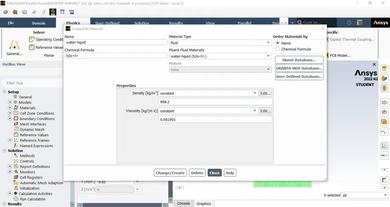
Create/Edit Materials

Air:

Density = 1.225 kg/m^3

Viscosity = 1.7894e-05 kg/m-s

Water:

Density = 998.2 kg/m^3

Viscosity = 0.001003 kg/m-s

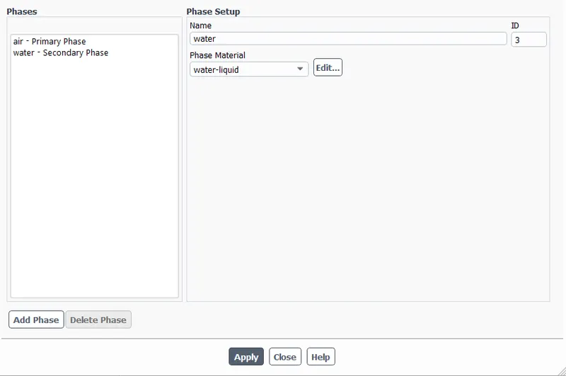
PHASES

List/show all phases

air - Primary Phase

water - Secondary Phase

II SOLUTION:

INITIALIZATION

Method --> Standard Initialization

Initialize at t = 0

Patch

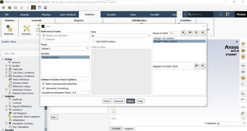
Phase --> water

variable --> volume Fraction

zones to patch --> water_water_surface

value -->1

Phase --> Air

variable --> volume Fraction

zones to patch --> air_air_surface

value -->0

III RESULTS

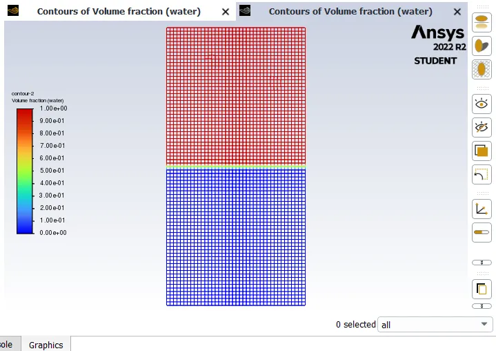
GRAPHICS

Contour --> New

options --Filled

contours of -->Phases

surfaces - select all surfaces

Display

IV SOLUTION

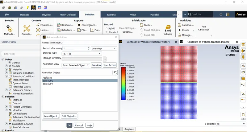
ACTIVITIES

Create --> solutions Animation

Animation object --> contour

PHASE 2

SLIMILARY TO PHASE 1

INITIALIZATION

Method --> Standard Initialization

Initialize at t = 0

Patch

Phase -->Air

variable --> volume Fraction

zones to patch --> air_air_surface

value -->1

Phase --> water

variable --> volume Fraction

zones to patch --> water_water_surface

value -->0

RUN CALCULATON

Time step size = 0.25

No. of Time Steps = 100

Solver - Pressure Based

Time - Transient

Gravity - enabled, y = -9.81 m/s^2

Multiphase - Volume of fluid

Viscous - Laminar

Material - Fluid - Air and Water

For Second part use Material - Air and User defined with density = 400 kg/m³, viscosity = 0.001 kg/m-s

Solution Initialization - Standard Initialization.

Phase - Water - Volume Fraction. Provide 1 for water surface and 0 for air surface.

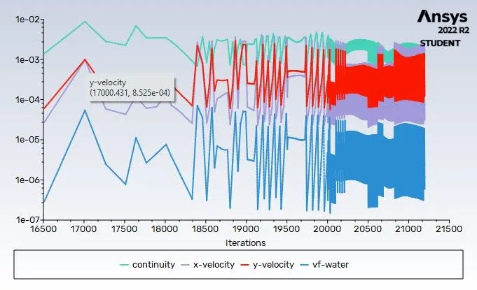
Fine meshing (element size = 20mm) (Water and Air)

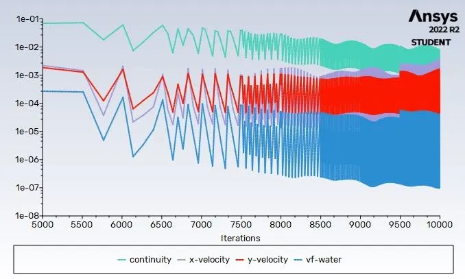
Fine meshing (element size = 20mm) (Water and User Defined Fluid)

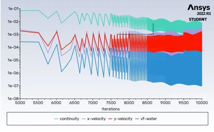
RESULTS:

Explain why a steady state approach might not be suitable for these types of simulation

• The steady state simulation is performed if we are concerned more about the final state results or the equilibrium state.
• In Rayleigh Taylor instability CFD model, we are more concerned to learn about the transition of the irregularities that starts developing when high dense fluid, water is suspended above low dense fluid, air under gravity effect.
• so, by using transient solver along with refined mesh of the model, we can compute the smooth transition of irregularities that takes place at the interface of the fluids. The final results for both the steady and transient state will be the same.

Define the Atwood Number. Find out the Atwood number for this case and explain how the variation in Atwood number affects the behaviour of the instability. How can we use the Atwood number to validate our simulation result

• Atwood number, abbreviated as A, is a dimensionless number in fluid dynamics used in the study of hydrodynamic instabilities in density stratified flows,
• it is defined as the ratio of the density difference between two adjacent fluids with a common interface to the sum of their densities. Atwood number is an important parameter in the study of Rayleigh–Taylor instability and Richtmyer–Meshkov instability.
• In Rayleigh–Taylor instability, the penetration distance of heavy fluid bubbles into the light fluid is a function of acceleration time scale,

A=ρ1−ρ2ρ1+ρ2">A=ρ1−ρ2ρ1+ρ2A=ρ1−ρ2ρ1+ρ2

where

ρ1">ρ1ρ1 = density of heavier fluid

ρ2">ρ2ρ2 = density of lighter fluid

For Atwood number close to 0, RT instability flows take the form of symmetric “fingers” of fluid; for Atwood number close to 1, the much lighter fluid “below” the heavier fluid takes the form of larger bubble-like plumes. In Rayleigh–Taylor instability, the penetration distance of heavy fluid bubbles into the light fluid is a function of acceleration time scale,

Atwood number for this case:

Part -1 (Water and Air)

A = 0.9975

Part -2 (Water and User defined fluid)

A = 0.4278

The calculated Atwood number is approximately equal to 1, and from the simulation results it is found that when high dense fluid water poured is upon low dense fluid air then formation of large bubble like plumes takes place which travels towards upward region in the form of waves and some gets trapped at the lower regions during the initial stage, which afterward try to move towards upper region and at the end, both phases gets separated with some diffusivity left at the middle portion between them. Thus the calculated Atwood number is validated for our simulation results.

CONCLUSION:

• The Rayleigh–Taylor instability is observed at the interface of two fluids, of different densities which occurs when the lighter fluid is pushing the heavier fluid due to which formation of shock waves at the interface takes place.

• Formation of air bubbles starts taking place, which compresses the heavy fluid around it, due to which shock waves of multidimensional fashion generates and it gets more stronger as it moves upwards.

• If the Mesh is refined from the baseline mesh, the simulation results become smoother. In case 2 and 3 we can see detail and smoother results as compared with baseline mesh.

• The formation of air bubbles that gets trapped at the lower region during the initial stage and then they travel towards the upper region generating shock waves. At the end of the simulation, it is to be observed that the two phases gets separated from eachother. some diffusivity between them is a volume fraction of air and water.