Week 5 - Rayleigh Taylor Instability

1. What are some practical CFD models that have been based on the mathematical analysis of Rayleigh Taylor waves? Explain how these mathematical models have been adapted for CFD calculations.
2. Perform the Rayleigh Taylor instability simulation for 2 different mesh sizes with the base mesh being 0.5 mm. Compare the results by showing the animations( Attach them from your google drive). Observe the differences in the animation and explain the effect of mesh size on simulation. Also, explain why a steady-state approach might not be suitable for these types of simulation.[ Choose Air and Water for this simulation]
3. Run one more simulation with water and user-defined material (density = 400 kg/m³, viscosity = 0.001 kg/m-s) for refined mesh.
4. Define the Atwood Number. Find out the Atwood number for both the cases and explain how the variation in Atwood number in the above two cases affects the behaviour of the instability.

Solution:

The Rayleigh–Taylor instability, or RT instability is an instability of an interface between two fluids of different densities which occurs when the lighter fluid is pushing the heavier fluid. Examples include the behaviour of water suspended above oil in the gravity of Earth, mushroom clouds like those from volcanic eruptions and atmospheric nuclear explosions, supernova explosions in which expanding core gas is accelerated into denser shell gas, instabilities in plasma fusion reactors and inertial confinement fusion.

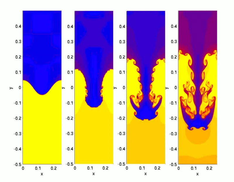
1. Some of the practical CFD models that have been based on the mathematical analysis of Rayleigh Taylor waves and how these mathematical models have been adopted for CFD calculations.

a) Saffman–Taylor instability:

The Saffman–Taylor instability, also known as viscous fingering, is the formation of patterns in a morphologically unstable interface between two fluids in a porous medium. This situation is most often encountered during drainage processes through media such as soils. It occurs when a less viscous fluid is injected, displacing a more viscous fluid; in the inverse situation, with the more viscous displacing the other, the interface is stable and no instability is seen. Essentially the same effect occurs driven by gravity (without injection) if the interface is horizontal and separates two fluids of different densities, the heavier one being above the other; this is known as the Rayleigh-Taylor instability.

b) Richtmyer–Meshkov instability:

The Richtmyer–Meshkov instability (RMI) occurs when two fluids of different density are impulsively accelerated. Normally this is by the passage of a shock wave. The development of the instability begins with small amplitude perturbations which initially grow linearly with time. This is followed by a nonlinear regime with bubbles appearing in the case of a light fluid penetrating a heavy fluid, and with spikes appearing in the case of a heavy fluid penetrating a light fluid. A chaotic regime eventually is reached and the two fluids mix. This instability can be considered the impulsive-acceleration limit of the Rayleigh–Taylor instability.

c) Mushroom cloud:

A mushroom cloud is a distinctive mushroom-shaped flammagenitus cloud of debris, smoke and usually condensed water vapor resulting from a large explosion. The effect is most commonly associated with a nuclear explosion, but any sufficiently energetic detonation or deflagration will produce the same effect. They can be caused by powerful conventional weapons, like thermobaric weapons, including the ATBIP and GBU-43/B Massive Ordnance Air Blast. Some volcanic eruptions and impact events can produce natural mushroom clouds.

Mushroom clouds result from the sudden formation of a large volume of lower-density gases at any altitude, causing a Rayleigh–Taylor instability. The buoyant mass of gas rises rapidly, resulting in turbulent vortices curling downward around its edges, forming a temporary vortex ring that draws up a central column, possibly with smoke, debris, and/or condensed water vapor to form the "mushroom stem". The mass of gas plus entrained moist air eventually reaches an altitude where it is no longer of lower density than the surrounding air; at this point, it disperses, drifting back down.

d) Kelvin–Helmholtz instability:

The Kelvin–Helmholtz instability typically occurs when there is velocity shear in a single continuous fluid, or additionally where there is a velocity difference across the interface between two fluids. A common example is seen when wind blows across a water surface; the instability constant manifests as waves. Kelvin-Helmholtz instabilities are also visible in the atmospheres of planets and moons, such as in cloud formations on Earth or the Red Spot on Jupiter, and the atmospheres (coronas) of stars, including the sun's.

2A. Rayleigh Taylor instability simulation for 2 different mesh sizes with the base mesh being 0.5 mm. Compare the results by showing the animations:

a) Geometry:

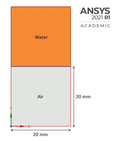
Share topology is enabled. SpaceClaim can share topology (face, edge, and vertex connections) between touching or intersecting bodies and surfaces in designs that are transferred to ANSYS.

Shared topology is the only way to achieve a conformal mesh where bodies meet, and is the only way to be certain that the intersection of bodies is meshed perfectly.

Case 1: Simulation with mesh size 0.5 mm:

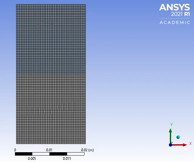
> Meshing Details:

• Mesh Type: Hexa
• Element Size: 0.5 mm

- Mesh Statistics:

• Nodes: 3321
• Number of Elements: 3200

> Setup:

• Model: Volume of fluid
  
  • Formulation: Implicit Method
• Phases:
  • Primary Phase: Air
  • Secondary Phase: Water
• Solver: Pressure Based
• 2D Space: Planar
• Time: Transient
• Fluid: Water and Air
• Viscous Model: K-Omega
  • K-Omega Model: SST
• Gravity Acceleration: -9.81 m/`s^2`

> Solution:

Once initialized (or calculated) the entire flow field, different values for particular variables are patched into different cells with respect to volume fraction.

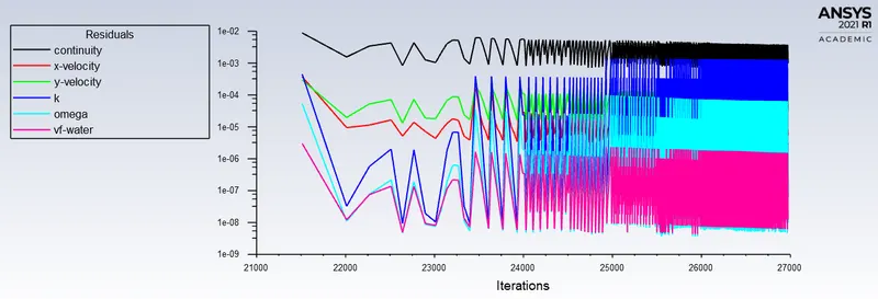
- Residuals Plot:

> Result:

- Volume Fraction Animation:

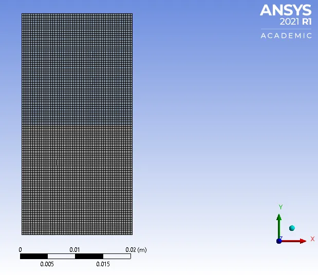
Case 2: Simulation with mesh size 0.4 mm:

> Meshing Details:

• Mesh Type: Hexa
• Element Size: 0.4 mm

- Mesh Statistics:

• Nodes: 5151
• Number of Elements: 5000

> Setup remains same as Case 1.

> Solution:

Once initialized (or calculated) the entire flow field, different values for particular variables are patched into different cells with respect to volume fraction.

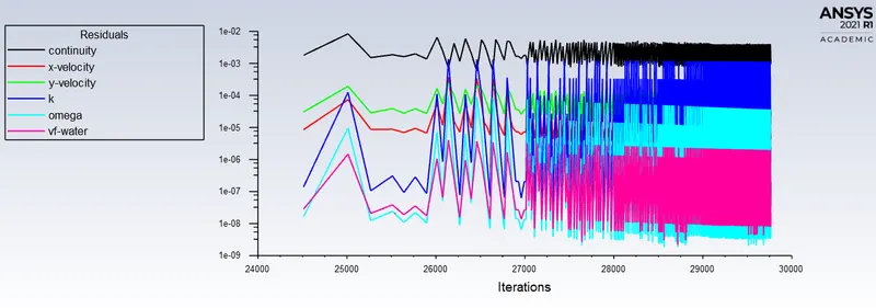
- Residuals Plot:

> Result:

- Volume Fraction Animation:

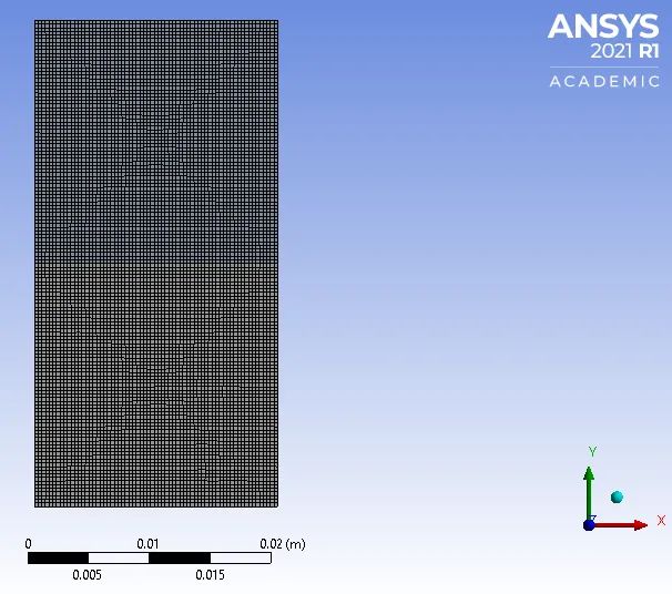
Case 3: Simulation with mesh size 0.3 mm:

> Meshing Details:

• Mesh Type: Hexa
• Element Size: 0.3 mm

- Mesh Statistics:

• Nodes: 9180
• Number of Elements: 8978

> Setup remains same as Case 1.

> Solution:

Once initialized (or calculated) the entire flow field, different values for particular variables are patched into different cells with respect to volume fraction.

- Residuals Plot:

> Result:

- Volume Fraction Animation:

2B. Effect of mesh size on simulation:

• The accuracy of volume fraction values of are enhanced in cases 2 and 3 comparatively, when meshes are refined further.
• The quality of animations are improvised by refining the mesh sizes and smoother results are obtained.
• Computation time in second and third cases are relatively higher as mesh is refined further. This might not be economical at certain cases.

2C. Why a steady-state approach might not be suitable for these types of simulation? [For Air and Water for this simulation]:

• Steady state is a state of process which does not change with respect to time, on the other hand Rayleigh Taylor Instability varies with respect to time. Rayleigh Taylor Instability CFD Models involves turbulent flow and are subjected to external environmental conditions.
• In transient method, we can also get the intermediate solution at a particular time step, whereas in we can get solution only at last iteration, but not in between. Also the computation time will be more in transient condition and then it requires more space.

3. Simulation with water and user-defined material (density = 400 kg/m³, viscosity = 0.001 kg/m-s) for refined mesh (Mesh size = 0.3 mm).

> Geometry:

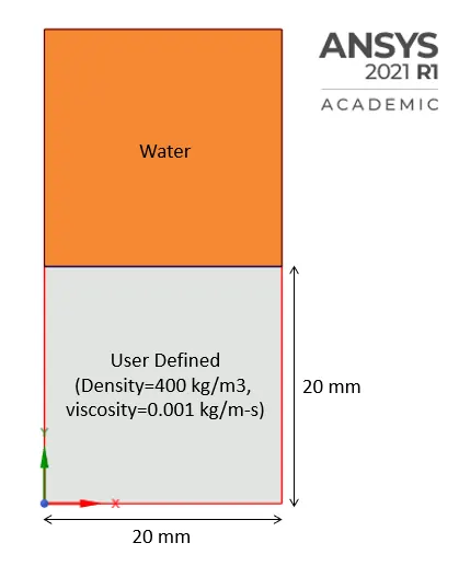
> Meshing Details maintained same as refined mesh from Case 3.

> Setup remains same as Case 1.

> Solution:

Once initialized (or calculated) the entire flow field, different values for particular variables are patched into different cells with respect to volume fraction.

- Residuals Plot:

> Result:

- Volume Fraction Animation:

4. Define the Atwood Number. Find out the Atwood number for both the cases and explain how the variation in Atwood number in the above two cases affects the behaviour of the instability.

Atwood Number is a dimensionless number that describes the density difference between two adjacent fluids with a common interface.

Atwood number`A = (rho_1-rho_2)/(rho_1+rho_2)`

where rho_1 = Density of Heavier Fluid

rho_2 = Density of Lighter Fluid

> Atwood number for Baseline mesh (Case 1) and refined meshes (Cases 2 and 3):

Density of Air = 1.225 kg`m^3`

Density of Water = 998.2 kg`m^3`

`A = (998.2-1.225)/(998.2+1.225)` = 0.9975

> Atwood number for water and user defined material with refined mesh:

Density of user defined material = 400 kg`m^3`

`A = (998.2-400)/(998.2+400)` = 0.4278

> Explain how the variation in Atwood number in the above two cases affects the behaviour of the instability.

• In case of RT instability simulation for water and air (with refined mesh), Atwood number (0.9975) is close to 1. For A close to 1, the much lighter fluid (air) "below" the heavier fluid (water) takes the form of larger bubble-like plumes which can be seen in the animation video correspondingly.
• In case of RT instability simulation for water and user defined fluid (with refined mesh), Atwood number (0.4278) is close to 0. Hence, RT instability flow takes the form of symmetric "fingers" of fluid which can be observed from the animation video respectively.