Week 5 - Rayleigh Taylor Instability

Aim: To Conduct the Rayleigh’s Taylor instability Waves using CFD simulation.

Objective:

1. What are some practical CFD model that have been on the mathematical analysis of Rayleigh Taylor waves ? In your own words, explain how these mathematically models have been adapted foe CFD calculations.
2. Perform the Rayleigh Taylor instability simulation for Two different mesh sizes with the base mesh being 0.5mm.Compare the results by showing animations(Attach them from your google drive). Observe the difference in the animations and explain the effect of mesh size on simulation .Also explain why a steady -state approach might not be suitable for these types of simulation [choose air and water for this simulation].
3. Run one more simulation with water and user-defined material (density=400kg/m^3, Viscosity=0.001kg/m-s)for refined mesh.
4. Define the Atwood Number . Find out the Atwood number for both cases and explain how the variation in Atwood number in the above two cases affects the behaviour of the stability.

Explanation:

1. The Rayleigh-Taylor instability, or RT instability is the instability of an interface between two fluids of different densities which occurs when the lighter fluid is pushing the heavier fluid. Example include the behaviour of water suspended above oil in the gravity of earth, Mushroom clouds like those from a volcanic eruption and atmospheric nuclear explosion , Supernova explosion in which expanding core gas is accelerated into denser shell gas , Instability in plasma fusion reactors and internal confinement fusion.
2. Water suspended a top oil is an everyday example of Rayleigh-Taylor instability,and it may be modeled by two completely plane-parallel layers of immiscible fluid, the denser on top of the less dense one and both subject to the earth gravity .The equilibrium here is unstable to any perturbation or disturbances of the interface,If a part of heavier fluid is placed downwards with a equal volume of lighter fluid displaced upwards , the potential energy of the configuration is lower than the initial state, Thus the disturbances will grow and lead to a further release of potential energy.As the more dense material moves downwards under the effect of gravitational field , and the less dense material is placed upwards . This was the setup as studied by Lord Rayleigh The important insight by G.I Taylor was his realization that this situation is equivalent to the situation , when the fluid are accelerated with in the less dense fluid accelerate into the more dense fluid, This occurs in deep underwater of the surface of an expanding bubble and in a nuclear explosion.

Types of instability and some practical CFD models that have been based on the mathematically analysis of Rayleigh Taylor waves.

Ritchmyer-Meshkov instability:

The Ritchmyer-Meshkov instability arises when a shock wave interacts with an interface separating two different fluids. it combines compressible phenomena, such as shock interaction and refraction with hydrodynamic instability, Including non-linear growth and subsequent transaction to turbulence,across a wide range of Mach numbers.

Plateau-Rayleigh Instability:

The Plateau-Rayleigh instability often just called as Rayleigh instability, explains why and how a falling stream of fluid breaks up into smaller packets with the same volume but less surface area . This fluid instability is exploited in the design of a particular type of ink jet technology where a jet of fluids is perturbed into a study stream of droplets.

Kelvin-Helmholtz Instability:

The Kelvin-Helmholtz instability can occur where there is velocity shear in a single continuous fluid or there is a velocity difference across the interface between two fluids . An example is an wind blowing over water . This instability manifests in waves on the water surface. More generally , clouds the oceans , Saturn's bands and the sun’s corona shows this instability

Geometry Setup:

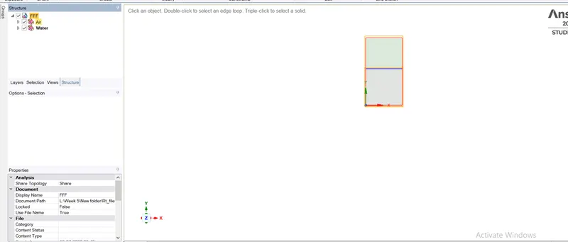
* Choose the fluent from the work bench setup, Edit Space claim to create Geometry.

*Choose XY plane to sketch 2D geometry , create a square of 20mm, and select pull tool to make a surface of that.

*Move the geometry to a new component and rename as AIR.

*Now create new geometry under the main design as water and create a square of 20mm right on top of the air square which creates a interface between the two boxes.

*Select the entire geometry for share preparation under the workbench and select share so that the interface can face information and conformal meshing can be achieved between the two phases.

Mesh setup:

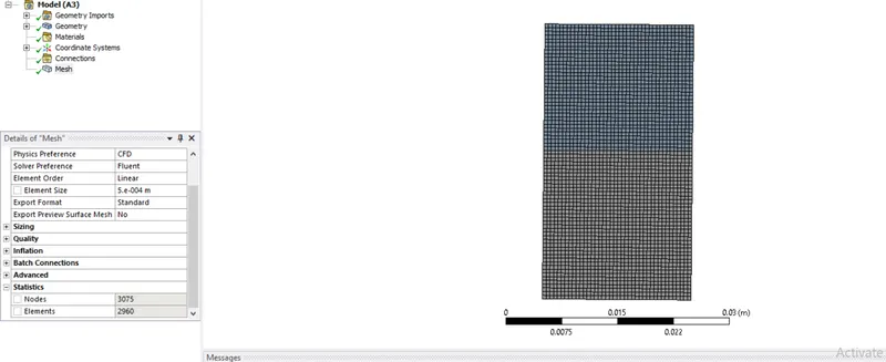
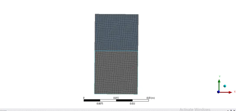
After creating the geometry open the mesh and generate the mesh with an element size of 0.5mm

Fluent setup:

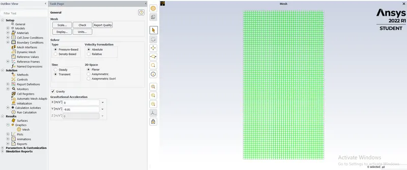
After updating the mesh open the fluent, here we set the general setting to pressure-based solver with transient time simulation because we have to see the interface collapse with the time . And select the gravity with a Y coordinate -9.81 m/sec.

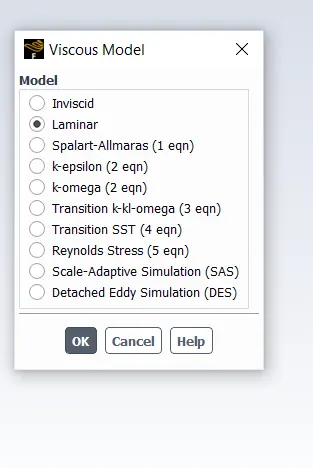
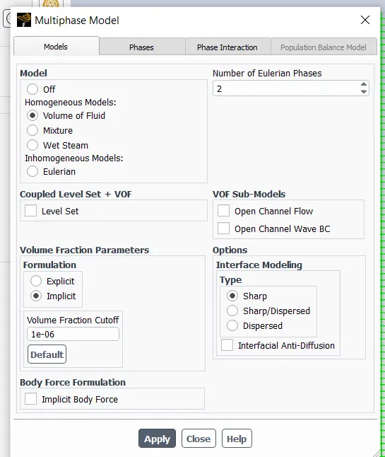
Under Physics use laminar in viscous flow and in the multi-phase select volume of the fluid model because here we designed to find out the position of the interface between two or more immiscible fluids.

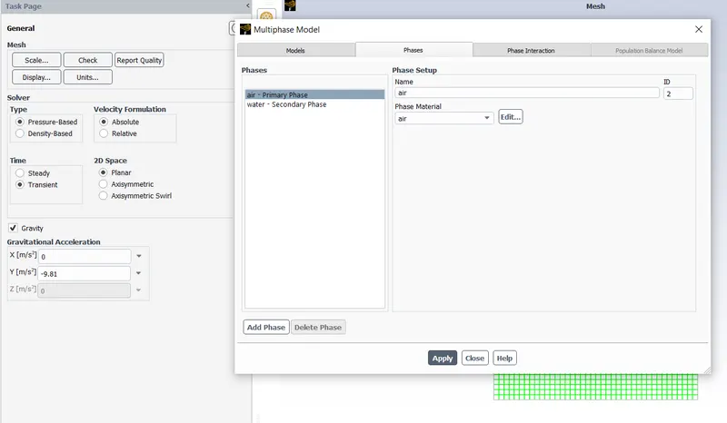
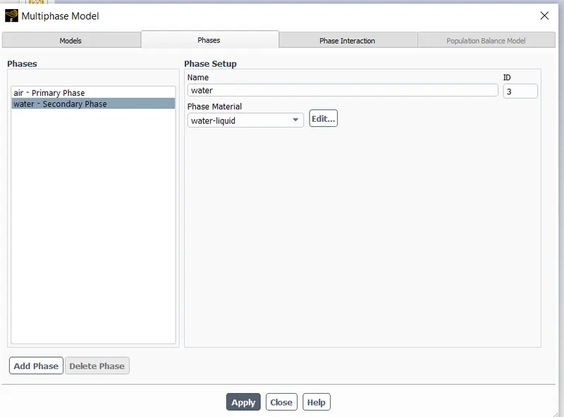
Add material water using fluent database and then assign the air as primary and water as secondary Phase.

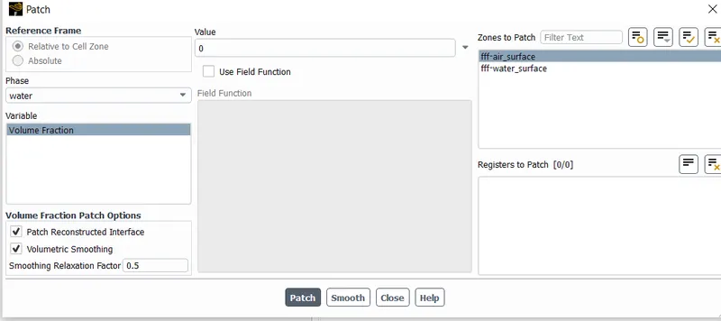
Initialize using standard initialization , then use the patch option to give the alpha value for water as1 and air as 0.

Create a contour for the phases and also the animation for the volume fraction of water .

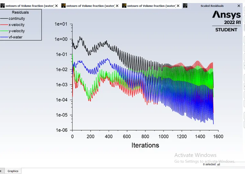
Now run the simulation with the time step size of 0.025 and 100 no of time steps ,if we encounter any error while running the simulation try reduce the momentum value in which under relaxation factors.

CFD Post: Use the post to see the fluid movement between the two phases.

CASE1:

Base Mesh with an element size of 0.5mm and having the fluid material air and water.

Elements=2940

Time step=0.025

No of Time step=100

Mesh:

Residual plot:

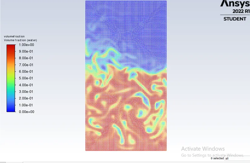
Contours of volume fraction:

CASE2:

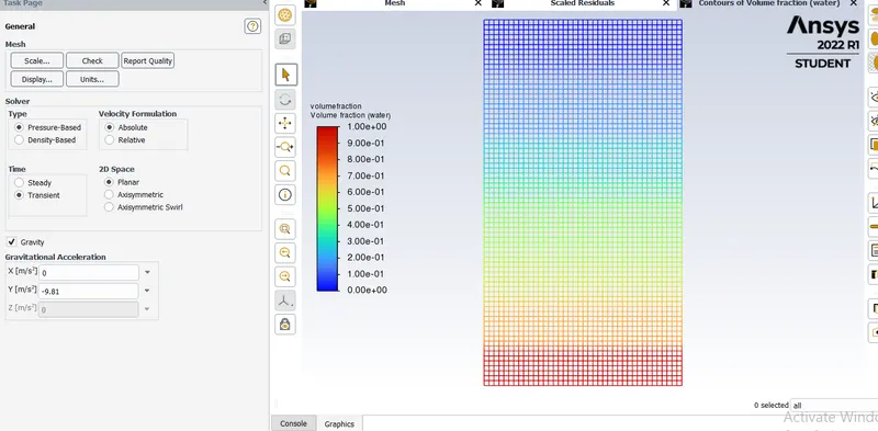
Refined Mesh with an element size of 0.3mm and having the fluid material air and water.

Elements=2940

Time step=500

No of Time step=0.01

Mesh:

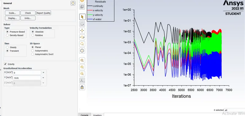
Residual plot:

Contours of volume fraction:

CASE3:

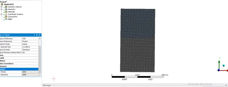
Refined Mesh with an element size of 0.3mm and having the user material and water.

Elements=8308

Time step=0.001

No of Time step=1000

Mesh:

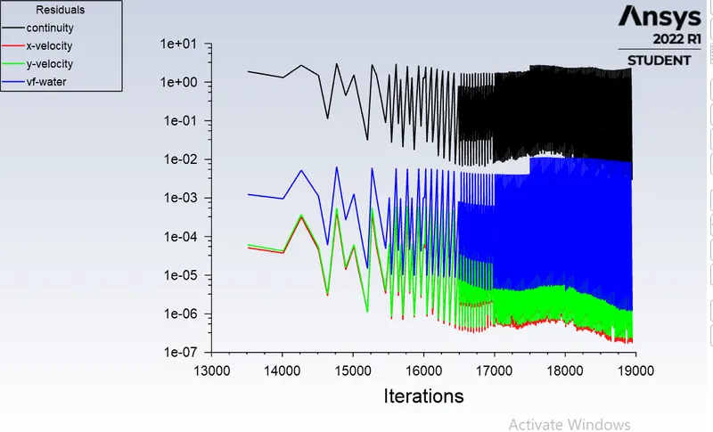
Residual plot:

Contours of volume fraction:

Video link:

https://drive.google.com/file/d/12YiwV4k977dhnSRWt0BYVREW6x8NSuB3/view?usp=sharing

Explanation:

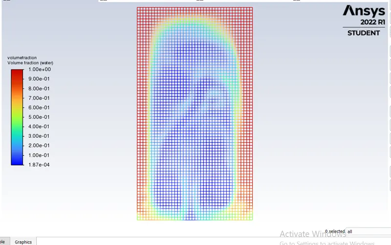
In the above challenge , the simulation starts with the state of hydraulic equilibrium , and Rayleigh Taylor instability is observed at the interface , When a lower density fluid pushes a higher density fluid due to formation of shock waves at the interface takes place, Formation of air bubbles starts takes place , which compress the heavy fluid around it Due to shock waves of multi dimensional fashion generates and it gets more stronger upward as it moves upward.

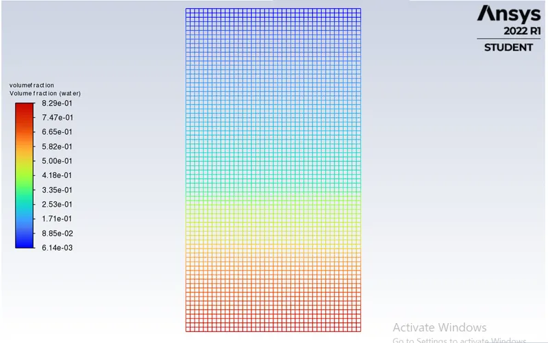
It is observed that the more we refine the mesh , the more the simulation results get smoother about the regularities that takes place at the interface of the two fluids, As higher density fluid replaces lower density fluid, the formation of air bubbles and vortex takes place, which travel towards the upward region with time.

In case-3 , We can see the more in detail results about the formation of waves and the formation of some air bubbles that get trapped at the lower region during the initial stage and then they travel towards the upward region, generating shock waves. At the end of the simulation , it is observed that the two phases get separated from each other though, we can see some difficulty between them which the volume fraction of air and water.

In the Rayleigh-Taylor instability , due to sudden collapse in the layer between the denser and lighter fluid spike generation takes place which is obviously time dependent , Hence using a steady state solver will not work as we are interested in the flow parameters with respect to time.

Atwood Number:

The Atwood Number (A) is a dimensionless number in fluid dynamics used in the study of hydrodynamic instabilities in density stratified flows. It is a dimension less density ratio as defined

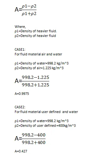
The difference in the fluids densities divided by the sum is defined as the Atwood Number (A).

For A close to 0, RT instability flow takes the form of symmetric “fingers” of fluids, For a close to 1,the much lighter fluid “below” the heavier fluid takes the form of larger bubbles -like plumes.

The behaviour RT instability on the variation of Atwood Number:

RT instability evolves in three distinct stages: Linear stability, Mushroom head (falling) or bubble raising formation, Long term evaluation due to bubble merging and mixing.For low Atwood number, bubble and Mushroom head shape is relatively Symmetrical , the disturbances of perturbations are linear for larger time , In Contrast for large Atwood number, bubble and Mushroom head shape is less symmetrical , Also it occurs rapidly at an accelerating rate which leads to a nonlinear growth rate.

Conclusion:

*From the above cases, we observe that finer mesh captures the instability better than the coarse mesh, but it takes more time for the heavier fluid to settle down. As computational time is long but produces result with better accuracy.

*Since the simulation involves capturing instabilities that are changing in a unpredictable manner as a function of time, the transient approach is preferred over the steady state approach.

*The Atwood no validates the CFD simulations as it is observed . In the case of water and air mixing, bubble formation takes place, whereas in the other case no bubble takes place.