Week 5 - Rayleigh Taylor Instability

Rayleigh Taylor Instability

Introduction:

In Multi phase, The dynamic variables of velocity, viscosity, pressure, and density are commonly employed to explain the movement of fluids under the gravitational field. Multi phase flows can be found in nuclear power facilities, food processing plants, and a variety of other places. Rayleigh Taylor Instability is one of the most fundamental examples. When a high density fluid is put on top of a low density fluid in a gravitational field, the Rayleigh Taylor Instability occurs. The RTI phenomenon was initially introduced by Rayleigh 1883 and later was observed for all accelerated fluids by Taylor 1950.When the density boundary is disrupted, hydro-static pressure is formed, forcing the heavier fluid to flow downhill and mix with the lighter one, with the amplitude of the disturbance first growing exponentially until saturating and generating the mushroom shape. When a heavier fluid is pushed below and an equivalent volume of lighter fluid is displaced higher, the potential energy of the system is reduced. This RTI has been used to solve a variety of issues, including mushroom clouds caused by volcanic eruptions, nuclear explosions, and the instability of plasma fusion reactors.

A significant range of numerical approaches, including as boundary integral methods, front tracking methods, volume of fluid methods, and phase field methods, have been introduced to simulate RTI. RTI was simulated using a semi-implicit moving particle approach that was well supported by experimental data. The multi-layered Richtmyer-Meshkov and RTI issues were simulated using the discontinuous Galerkin approach.

To mimic RTI of the immiscible two phase in-compressible fluid, the multi phase moving particle semi-implicit (MMPS) with periodic boundary conditions was used. The effect of initial perturbation wavelength, surface tension and Atwood Number was investigated in the single mode RTI problem and it was observed that the numerical results were in good agreement with the analytical results

Rayleigh–Taylor instability

It is an instability of an interface between two fluids of different densities which occurs when the lighter fluid is pushing the heavier fluid.

Examples include the behavior of water suspended above oil in the gravity of Earth, mushroom clouds like those from volcanic eruptions and atmospheric nuclear explosions, supernova explosions in which expanding core gas is accelerated into denser shell gas, instabilities in plasma fusion reactors and inertial confinement fusion.

Kelvin-Helmholtz instabilities

It occurs when there is velocity shear in a single continuous fluid or a velocity difference across the interface between two fluids. Kelvin-Helmholtz instabilities are visible in the atmospheres of planets and moons, such as in cloud formations on Earth or the Red Spot on Jupiter, and the atmospheres (coronas) of the Sun and other stars.

Richtmyer–Meshkov instability

It occurs when two fluids of different density are impulsively accelerated. Normally this is by the passage of a shock wave. The development of the instability begins with small amplitude perturbations which initially grow linearly with time. This is followed by a nonlinear regime with bubbles appearing in the case of a light fluid penetrating a heavy fluid, and with spikes appearing in the case of a heavy fluid penetrating a light fluid. A chaotic regime eventually is reached and the two fluids mix. This instability can be considered the impulsive-acceleration limit of the Rayleigh–Taylor instability.

However, in order to mimic the evolution of RTI's interface, the current work uses the Finite Element approach. The 2D geometry is created in Space claim and a computational mesh is developed in this study. The meshing file was imported into Fluent, and a grid dependence test was run, with the results of the RTI inter-facial evolution collected and compared at various flow periods. The RTI's governing equations were a modified version of the Naiver-Stokes equation and the Cahn-Hilliard equation.

Geometry:

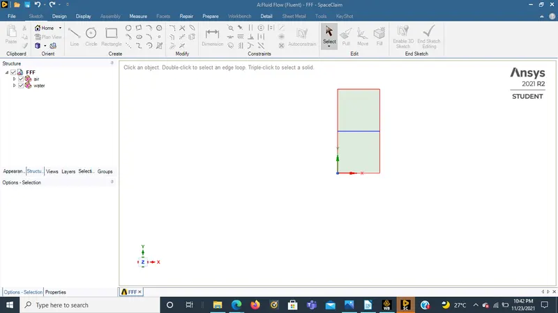
At first, geometry is created as square boxes and converted to surface using Pull tool and share topology is turned on. The geometry was created in space claim and it involves no other importing of CAD models. We used bottom surface body as air and upper surface body was water-liquid(H₂O).

Mesh Details:

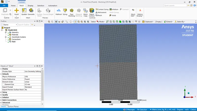
Case 1A:

Nodes: 3321

Elements: 3200

Mesh Size: 0.5mm

CFD Case Setup

• Pressure based solver and Absolute velocity is used.

• Transient-state Calculation is performed.

• Compressible fluid flow is chosen.

• Gravity is enabled in -ve Y axis (-9.81m/s)

• Multi phase Model is turned on along with Volume of Fluid and number of Eulerian phases is chosen as 2 and Implicit scheme is selected.

• Viscous model-Laminar is used.

• Cell zone selected as Fluid-air;water-surface:water-liquid

• Patching of the volume fraction of the two phases is performed before the start of simulation. Phase used for patching was water and volume fraction of 1 is taken for water surface and 0 for air surface.

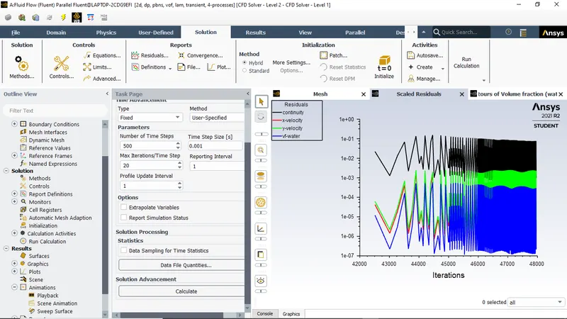
• In Pressure velocity coupling SIMPLE scheme is used. For the momentum second order upwind scheme is used and for pressure, PRESTO is selected. For the transient formulation first order implicit scheme is chosen for better results and for stability and convergence of the residuals.

https://youtu.be/IHdqNtlfsFQ

Post-processing Results :

The post processing was done in CFD Fluent.

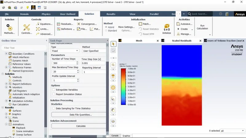
For Case 1A: The transient case was run for 3210 time steps with a Time step size of 0.0025. A more clearer settled fluids are observed. We can observe from the water volume fraction how the air has moved upwards while the water settles down.

At first the fluids behave linearly and we can observe small linearity sinking going on between them, slowly the chunky bubbles from the higher density fluid on top settles down. This can be identified from the highest mesh case resulting in finest behavior of the instability for this condition. At t = 0, the small enough, initial perturbation in flow can be described by a smooth function. We observe the disturbance in flow from smooth to turbulent growth has been observed (at t = 0.5 to t = 9). We also observed the transition of a single globule into lots of deformed globules with with lots of turbulence along with some breakup and penetration of heavier fluid into the lighter one. These breakups which seems at t = 0.11 vanishes as time proceed as in t = 2.253, showing the phenomena of Rayleigh-Taylor instability. At t = 0.349 and t = 2.7725, it is clear that the falling fluid is rolled up. In our result, finally the heavier fluid has settled down completely at 𝑡 = 7.7 𝑠 or we can say it is in the verge of complete settling. It shows the 2D-Rayleigh Taylor Instability simulation having the contours of two phase mixture model. At later time we observe the formation of low density bubbles and its rise into the high density phase whereas the high density globules sinks at the edges of the domain of the simulation into the light fluid. With the time evolution, the interface gets smeared due to numerical diffusion within the interfaces.

Case 1B:

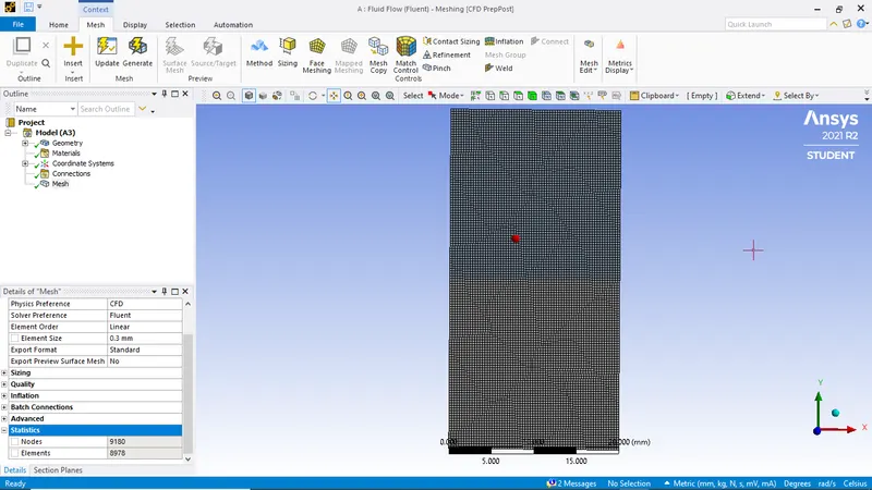
Mesh Details:

Nodes: 9180

Elements: 8978

Mesh Size: 0.3mm

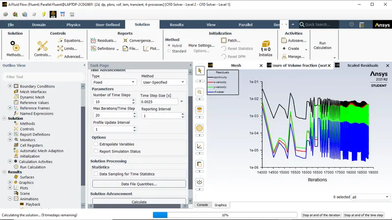
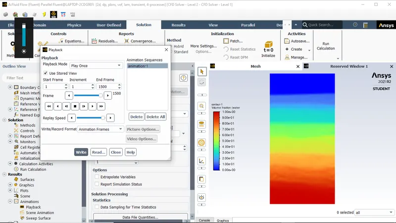
https://youtu.be/NpBpb7Es5Cw

Case 1C:

Mesh Details:

Nodes: 20301

Elements: 20000

Mesh Size: 0.2mm

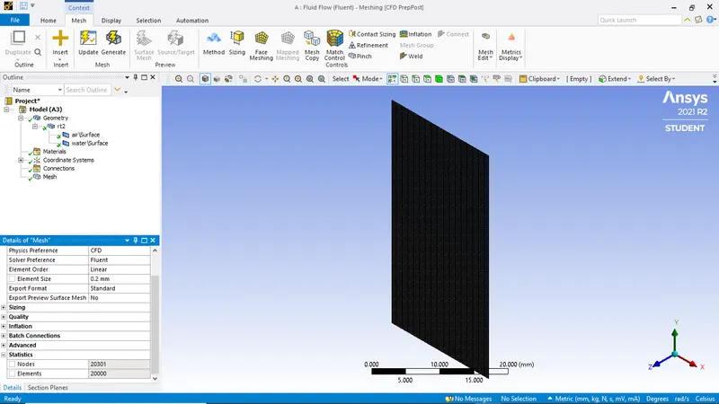
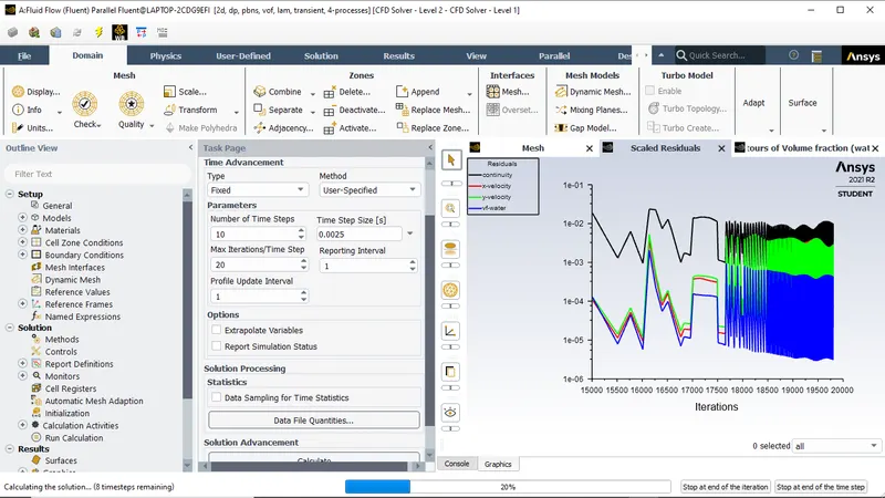
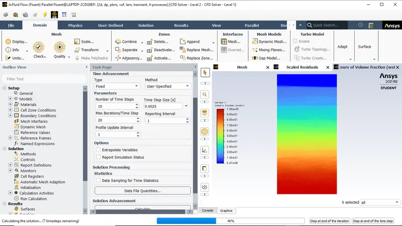
https://youtu.be/Vcp0LS4q3_0

By observing the three cases, The shape of the globules deforming as flow time progresses actually varies with the meshing. The volume fraction in simulations on different meshes at a particular flow time shows the interface thickness is smaller on finer mesh.

Case 2:

In this case we used the refined mesh as 0.2mm with 2000 iteration and 0.0025 time steps. The results are mention below.

Here we change the density of water to 400kg/m³.

Viscosity is 0.001kg/m-s.

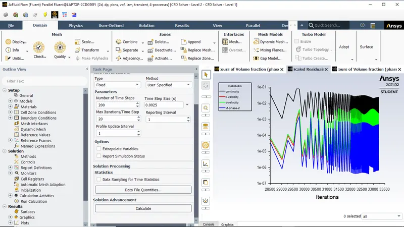
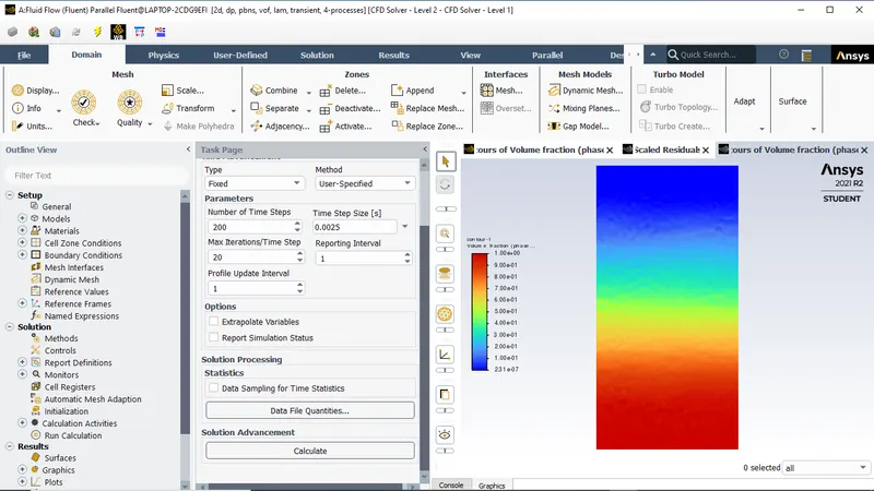
https://youtu.be/TYZeusrTeas

Atwood number:

The Atwood number (A) is a dimensionless number in fluid dynamics used in the study of hydrodynamic instabilities in density stratified flows. It is a dimensionless density ratio defined as

A =

ρ₂ – Density of heavier fluid

ρ₁ – Density of lighter fluid.

Case 1:

Density of heavier fluid (water) = 998.2 kg/m³

Density of lighter fluid (air) = 1.225 kg/m³

A= = = 0.9975.

Case 2:

Density of heavier fluid (water) = 998.2 kg/m³

Density of lighter fluid (User material) = 1.225 kg/m³

A= = = 0.42783.

Conclusion:

Rayleigh Taylor flimsiness was seen at the interface of the liquids with various thickness affected by gravity.The lower thickness liquid pushes the higher thickness liquid above it. The heavier liquid which is water, for this situation, comes at the base and replaces the air from the bottom. The development of air bubbles happens which moves upward. The network refinement prompts better reproduction of the Rayleigh Taylor precariousness. All the insecurity and the abnormalities that happen at the interface are better pictured as we refined the mesh. In every one of the cases the lower thick liquid pierces into the high-thickness liquid as it is by all accounts the proliferation of shock wave.In case 1A at the interface, we can see that a few unsettling influences are shaped as time elapsed the huge aggravation is framed its powers into the high thick liquid like a shock wave. In case 1B at the interface, we can see the unsettling influences which are more than case 1 pushing through the high thick liquid mushroom-like construction is framed and the arrangement of air pockets can be seen around the mushroom structure.In case 1C at the interface aggravations are seen in more detail as many air pockets and the development of vortices are can be plainly seen.After playing out the 1C case arrangements with individual base matrix measures the case-1A& 2 we can see that there were just minor changes in the post-handling results showing us that the case had combined. The better the cross section the more prominent the chance of exact stream expectation. Here Case 1C has the best cross section of all. So would we be able to take information from case 1C since it will have a precise recreation result.