Week 5: Prandtl Meyer Shock problem
Prandtl-Meyer Shock Simulation
Introduction
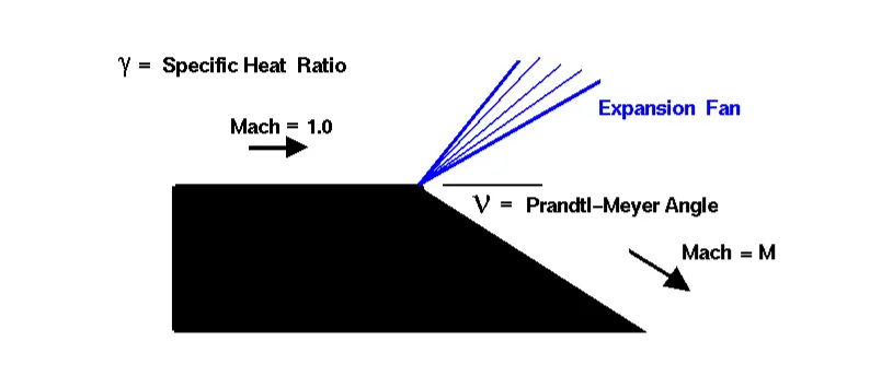
Movement of object through gas causes its molecules to deflect. Given the speed of the object is less than the speed of sound in the gas, the density of the gas remains constant and the flow of gas can be described by conserving momentum and energy.
As the speed of the objects increases approaching the speed of sound, effects of compressibility of the gas must be considered. The density of the gas varies locally as the gas is compressed by the moving object. When an object moves faster than the speed of sound, and there is an abrupt decrease in the flow area, leading to generation of shock waves. If the flow area increases, however, a different flow phenomenon is observed. If the increase is abrupt, we encounter a centered expansion fan.
There are some marked differences between shock waves and expansion fans. Across a shock wave, the Mach number decreases, the static pressure increases, and there is a loss of total pressure because the process is irreversible.
Through an expansion fan (also a topic of present study), the Mach number increases, the static pressure decreases and the total pressure remains constant. Expansion fans are isentropic.
The calculation of the expansion fan involves the use of the Prandtl-Meyer function. This function is derived from conservation of mass, momentum, and energy for very small (differential) deflections.
`nu = sqrt({gamma + 1}/{gamma - 1}) tan^-1sqrt(({gamma -1}/{gamma + 1})(M^2 - 1)) - tan^-1sqrt((M^2 - 1))`
Where `nu` is the Prandtl-Meyer Function, m is the Mach No. and Gamma is the the ratio of specific heats of gas(constant pressure/volume).
The physicality of Prandtl-Meyer function is its relation with the angle of expansion such that it can transform incoming Mach 1 to a desired mach No.
Increase in mach no. through the outlet depends on inlet mach no, and angle of expansion
Boundary Conditions:
Types of boundary condition:
- Dirichlet Boundary Condition
It specifies the values that the solution has to take along a boundary of the domain. It can be either slip or no-slip boundary condition, in the terms of velocity filed variable. In slip boundary condition, velocity along the boundary is not set to zero, instead only the velocity normal to boundary is set to zero.
For No-Slip boundary condition, both velocity normal and parallel to the boundary is set to zero.
- Neuman Boundary Condition
When imposed on an ordinary (ODE) or a partial differential equation (PDE), it specifies the values that the derivative of a solution is going to take on the boundary of the domain.
- Robin Boundary Condition
It consists of a linear combination of the values of the field and its derivatives on the boundary.
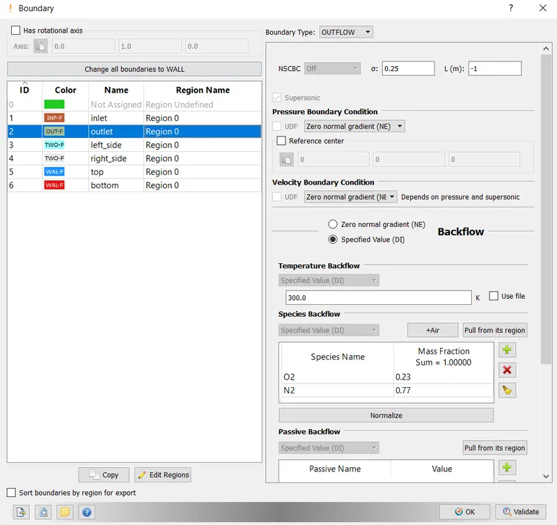
The pressure outlet boundary condition with a specified gauge pressure is only applicable in subsonic flow problems. For the supersonic flow, the pressure needs to be extrapolated from the interior grid points. Therefore, for outflow, Neuman boundary condition is applicable, which approximate the solution using derivatives of interior variables.
Objective
The objective of present study includes set up of steady-state simulation of Prandtl-Meyer Problem with a focus on observing the effect of increasing temperature sensitivity via adaptive mesh generation on shock location and total cell count.
Outline
In order to achieve the objective of our study, the simulation has been divided into 3 cases as follows:
Case 1:
SGS = 0.05K
Case 2:
SGS = 0.03K
Case 3:
SGS = 0.01K
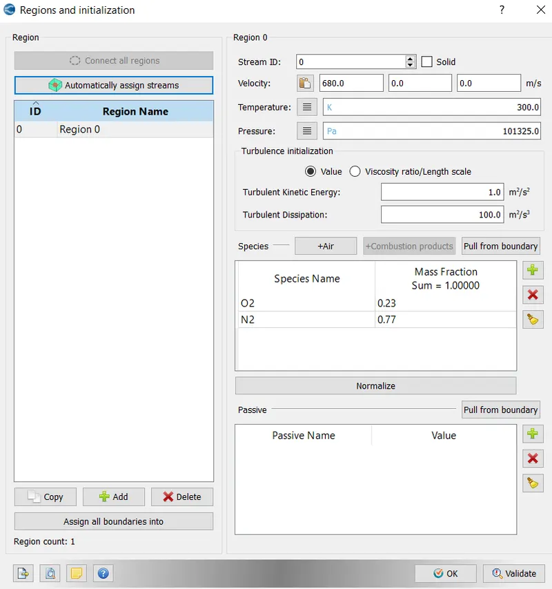
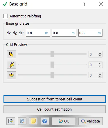
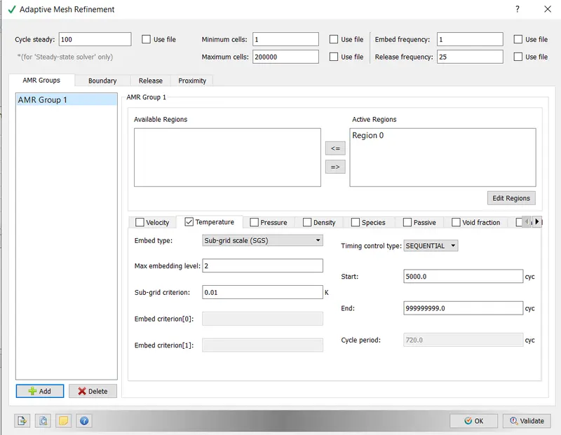
Velocity at inlet of all the three cases is 680 m/s which is twice the speed of sound. The base grid size is of 0.8 m with a final embedding of 2 levels. That is, the minimum grid size is of 0.2m.
Simulation
Material
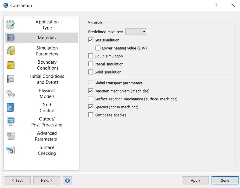
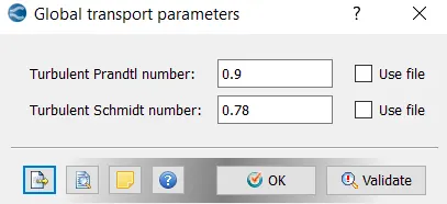
Air with the default transport properties has been choosen for the simulation
Geometry and boundary names
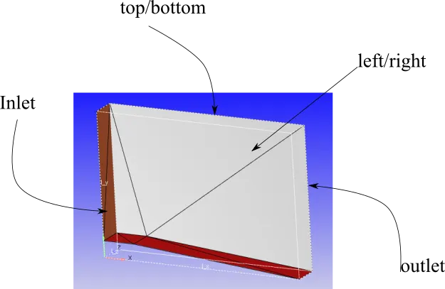
As described in the geometry section, the boundaries are devided into top/bottom inlet, outlet and left/right side
inlet has been given inflow boundary condition with a velocity of 2 mach in x direction. Since we are not dealing with any chemical reaction, inlet and outlet species are kept same.
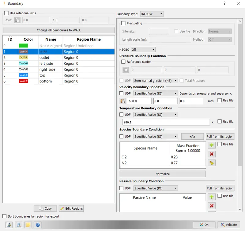
outlet has been given outflow boundary condition with pressure and velocity boundary condition to be Neuman Boundary condition.
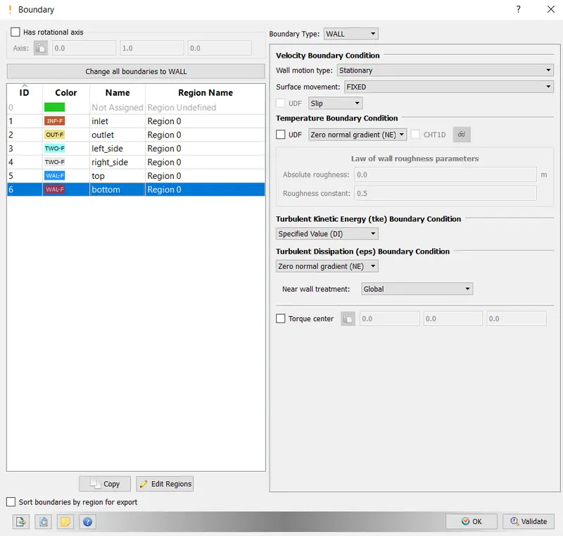
left and right side has been diven 2-D boundary condition.
Top and Bottom has been given wall type boundary with fixed geometry.
Region and Initialization
Solver
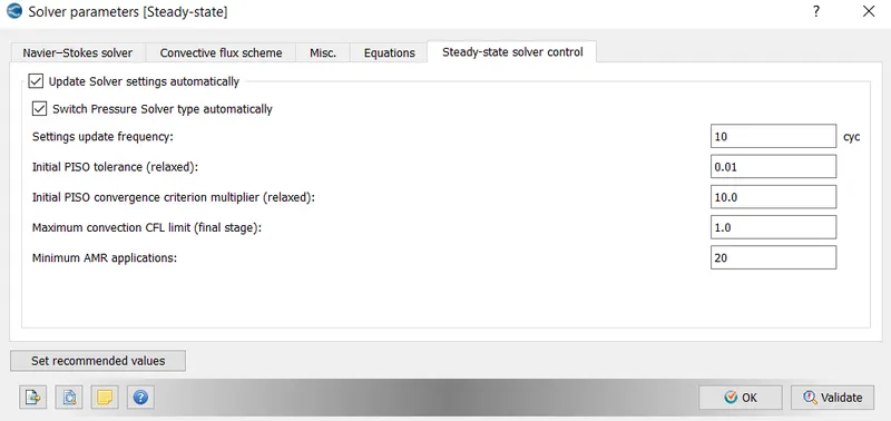
Since the simulation is of steady-state type, a steady state solver hase been selected.
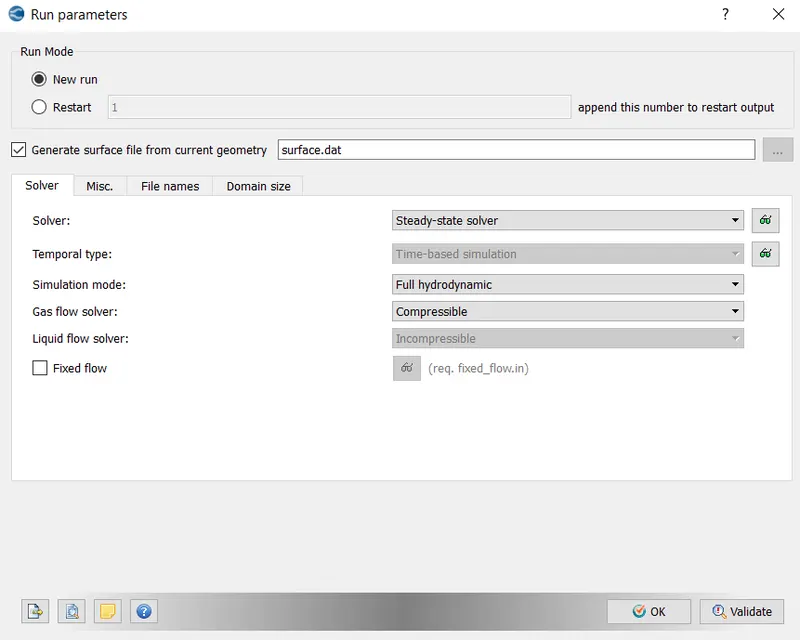
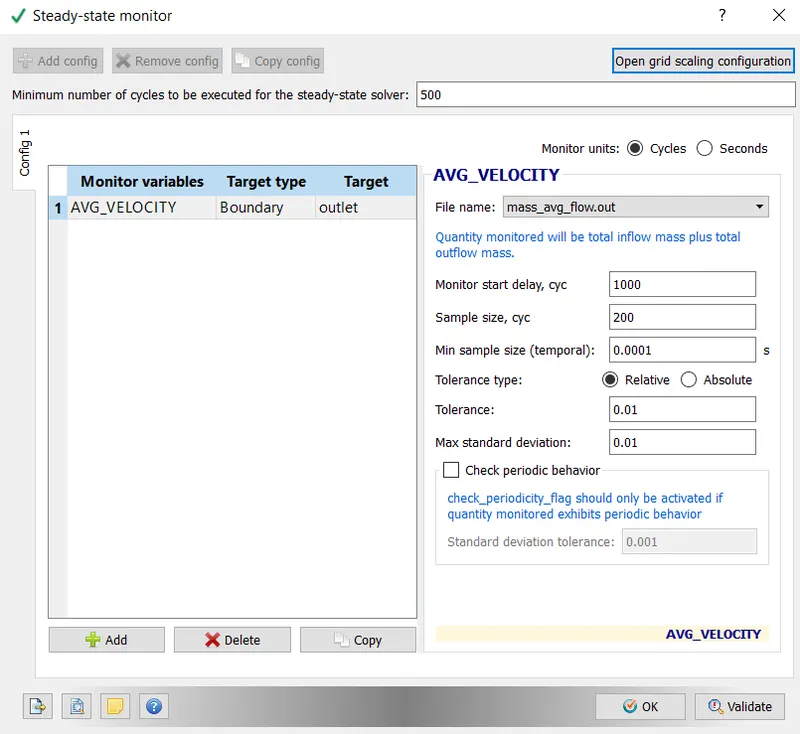
Average Velocity is set to be the monitoring variable at the outlet boundary.
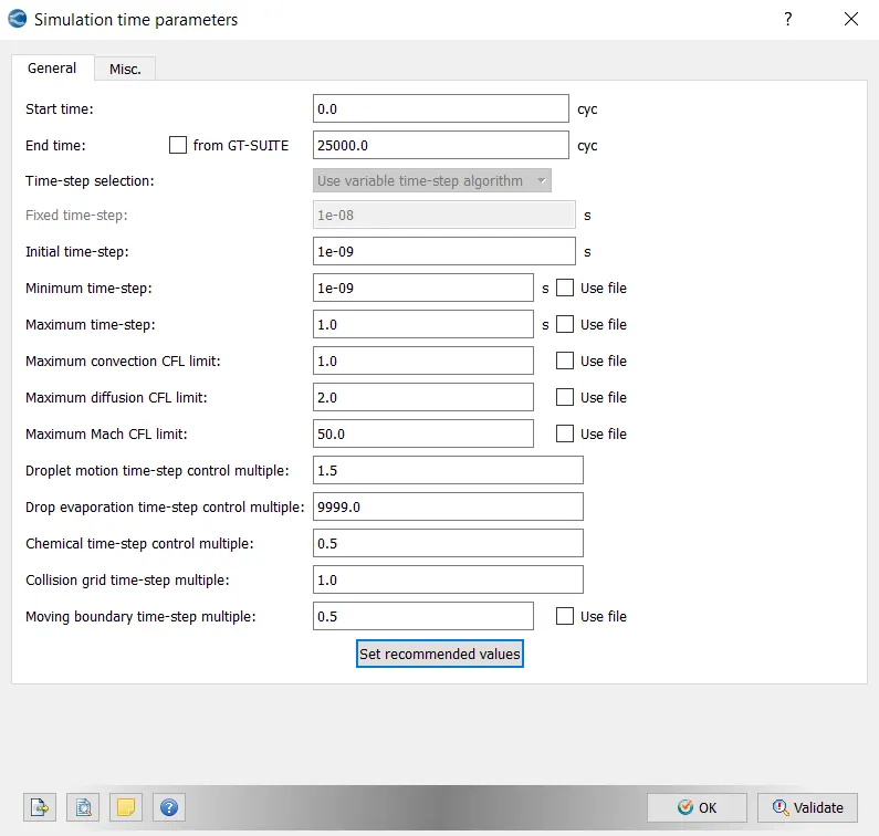
A maximum of 25000 cycle has been chosen with maximum convection cfl to be 1.
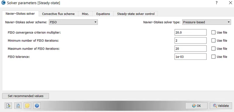
Pressure based somver has been used in the present study. The temperature extrapolation error can be solved using a low final cfl no.
Grid
A base grid of 0.8m has been substituted.
Adaptive mesh refinement
Temperature based adaptive mesh refinement stategy has been introduced, with a varing SGC.
Result and Discussion
As specified in the outline of the project, to observe the effect of SGS in total cell count and shock location, the simulation is divided into 3 cases.
Effect of SGS on Total cell Count
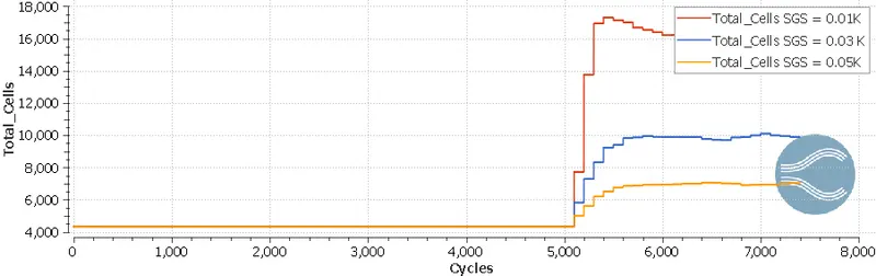
Effect of SGC on the mesh generation.
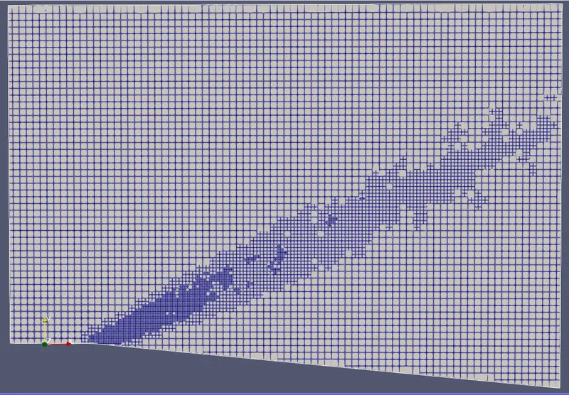
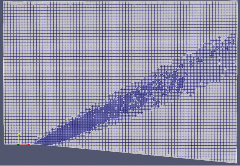
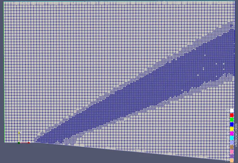
Mesh Grid
Case 1 : SGS = 0.05K
Case 2 : SGS = 0.03K
Case 3 : SGS = 0.01K
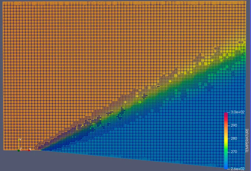
Temperature Contour Plot
Case 1: SGS = 0.05K
Case 2: SGS = 0.03K
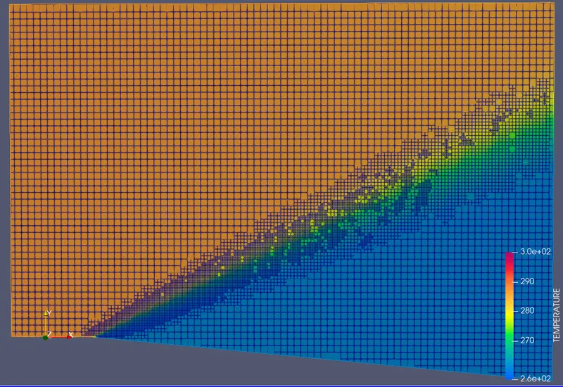
Case 3: SGS = 0.01K
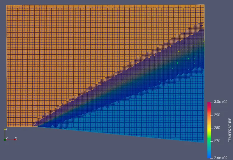
Conclusions:
Increase in Sub grid sensitivity or decrease in the value of sub-grid criterion leads to finer mesh. Since the lower limit of grid size is defined to be two orders below the base mesh, the smallest size would be of 0.2m.
Since the grid gets finer over large area, total cell count increases as we decrease the value of sub-grid criterion. This also leads to utilization high computation time and memory.
With increase in sensitivity with temperature, using adaptive meshing the shock line is clearly distinctive in temperature contour, with area under refined region being broad.