Prandtl Meyer Shock problem

Aim:-

• Explain shock wave and its interaction with boundary layer along with its applications.
• Setup the simulation for the Prandtl Meyer shock problem.
• Find out the effect of the SGS parameter on shock location and show the effect of SGS temperature value on cell count and the shock location.
• Create the animation with the help of the Paraview.

Objective:-

• Literature search on shock wave boundary condition with its use.
• Describe what is shock wave is and the physics behind the shock wave.
• Set up the Prandtl Meyer simulation setup.
• Simulate the simulation with different SGS parameters.
• Also, simulate the setup with mach number lower than 1 (100m/s).
• Show the effect of SGS temperature value on the cell count.
• Create animations with all SGS parameters to show its effect.

Shock Wave:-

As an object moves through a gas, the gas molecules are deflected around the object. If the speed of the object is much less than the speed of sound of the gas, the density of the gas remains constant and the flow of gas can be described by conserving momentum and energy.

As the speed of the object increases towards the speed of the sound, we must consider compressibility effects on the gas. The density of the gas varies locally as the gas is compressed by the object.

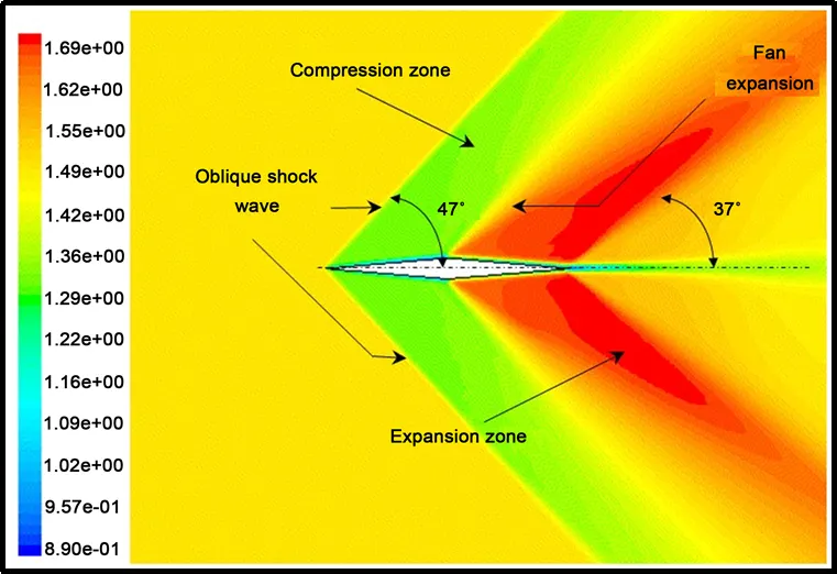
When an object moves faster than the speed of sound, and there is an abrupt decrease in the flow area, shock waves are generated.

Expansion Fan:-

If the flow area increases, however, a different flow phenomenon is observed. If the increase is abrupt, we encounter a centered expansion fan.

The difference between Shock Waves and Expansion Fans:-

• Across a shock wave, the Mach number decreases, the static pressure increases, and there is a loss of total pressure because the process is irreversible.
• Through an expansion fan, the Mach number increases, the static pressure decreases, and the total pressure remain constant.

The calculation of the expansion fan involves the use of the Prandtl-Meyer function. This function is derived from the conservation of mass, momentum, and energy. For very small (differential) deflections. The Prandtl-Meyer function is denoted by the Greek letter nu on the slide and is a function of the Mach number M and the ratio of specific heats `gamma` of the gas.

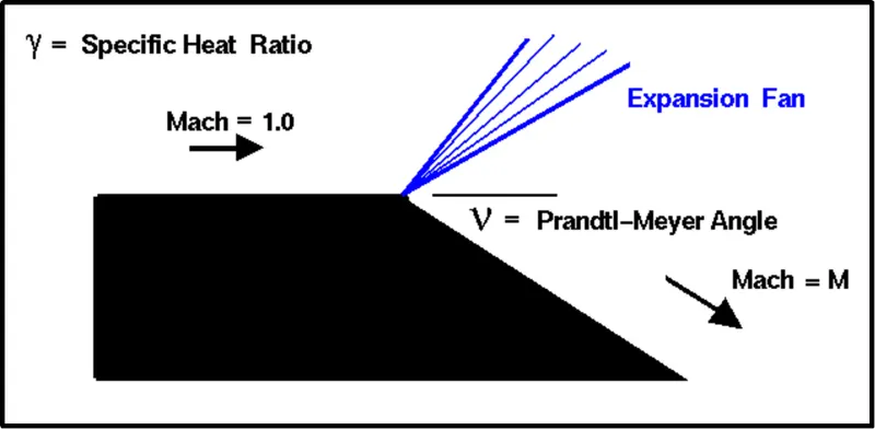
As mentioned above, the Mach number of a supersonic flow increase through an expansion fan. The amount of the increase depends on the incoming Mach number and the angle of the expansion. The physical interpretation of the Prandtl-Meyer function is that it is the angle through which you must expand a sonic (M=1) flow to obtain a given Mach number. The values of the Prandtl-Meyer function are therefore called the Prandtl-Meyer angel.

Interaction of Shock Wave with boundary layer:-

• Shock wave interactions are usually classified according to how the shock is generated.
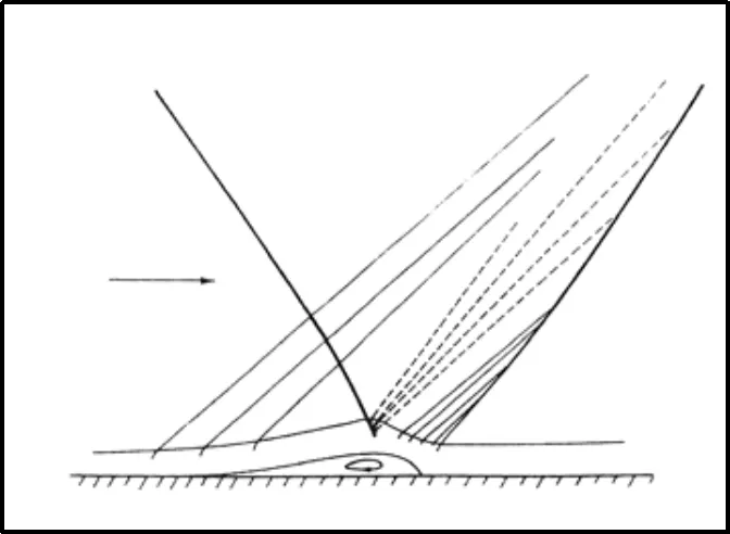
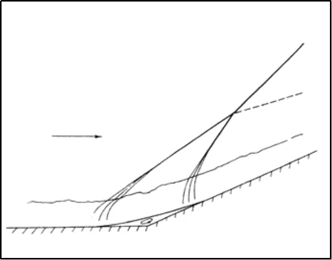
• For shock wave-boundary layer interactions, the shock may impinge on the layer from an external source (an incident shock interaction), or the shock may be generated by the same surface that generated the boundary layer (a compression surface or compression corner interaction).
• In three-dimensional interactions, the shock may be generated by a sharp fin placed at an angle of attack to the incoming flow, by a blunt fin where the leading edge has a finite radius of curvature, or by a cone or other protrusion rising from the surface.
• Interaction between shock wave and boundary layers incident oblique shock:

• Interaction between shock wave and boundary layers compression corner interaction:-

• In addition, the Mach number plays a crucial role in governing the in-viscid flow-field. For example, as the Mach number increases for a given shock generator configuration, the in-viscid shock may change from being detached to being attached, producing large changes in the near field.
• Even if the in-viscid shock is attached, the reduced Mach number within the boundary layer may cause detachment at some point, and this can change the entire flow pattern.
• Variations in Reynolds number will also play a role, but for fully-turbulent flows, its influence appears to be relatively minor because most interactions are pressure-dominated.

Boundary Definition:-

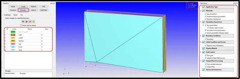
• First, the model was scaled with a factor of 0.001.
• Then the inlet, outlet, top-bottom wall, and front-back symmetry boundary names were provided for boundary definition.
• The below screen captured picture shows the boundary definition, scaled length or bounding box, and the setup tree of the simulation.

Simulation Setup/ Case setup:-

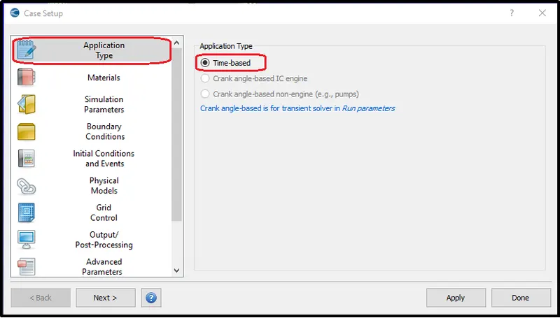
Application type:-

In the 'Application Type" section selects the "Time-based" application and click apply and done. later, we will get the option for a steady flow solver. It will show us a setup tree.

Material Definition:-

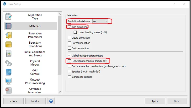
In this simulation, we simulated the results for compressible flow with fluid air.

Simulation Parameters:-

Run Parameters:-

This is a steady-state simulation, so the steady-state solver type was selected with simulation mode Full hydrodynamic using gas flow solver as compressible.

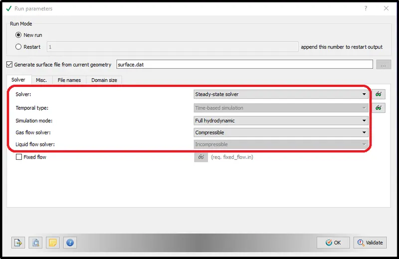
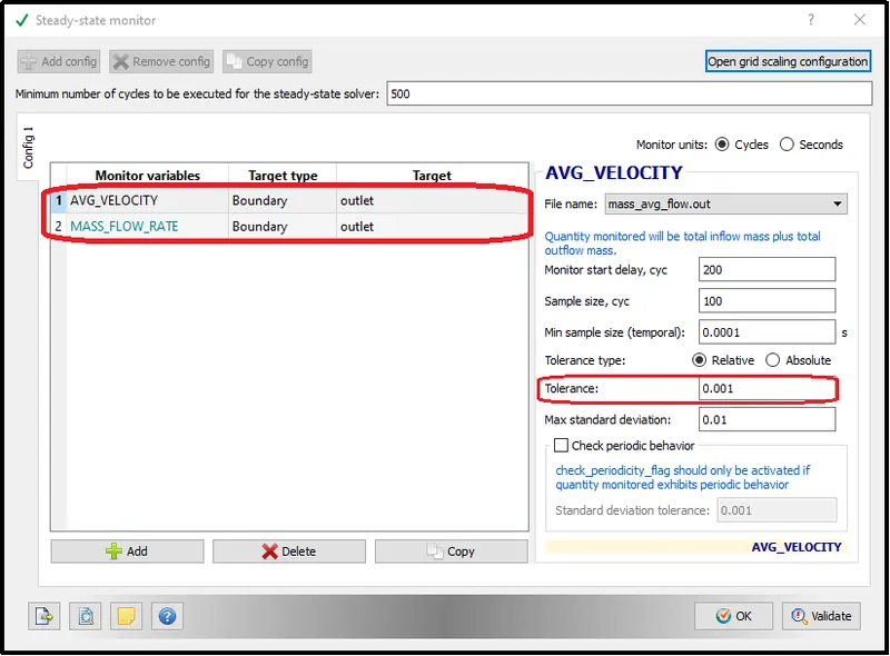
To monitor our results and converge our results with proper tolerance, the steady-state monitor box was checked. This gave us the option to control the accuracy of our results.

Steady-state monitor:-

In Steady-state monitor input two-parameter were monitored - one was Velocity at the outlet and another was mass Flow rate at the outlet. Tolerance for both was set as 0.001.

Simulation time parameters:-

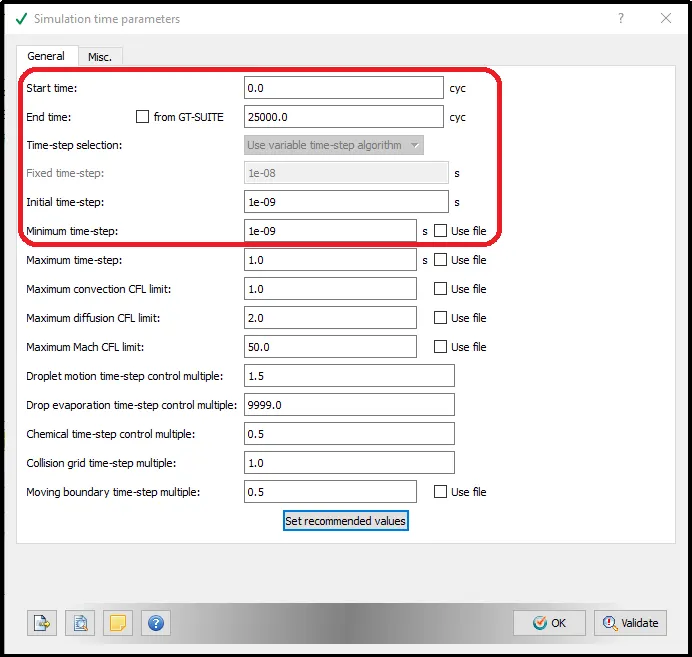
The cycle range was set for 0 - 25000 cycles with the initial time step and a minimum time step of 1e-09. Value of maximum time-step and maximum convection CFL limit set for 1.

Solver Parameters:-

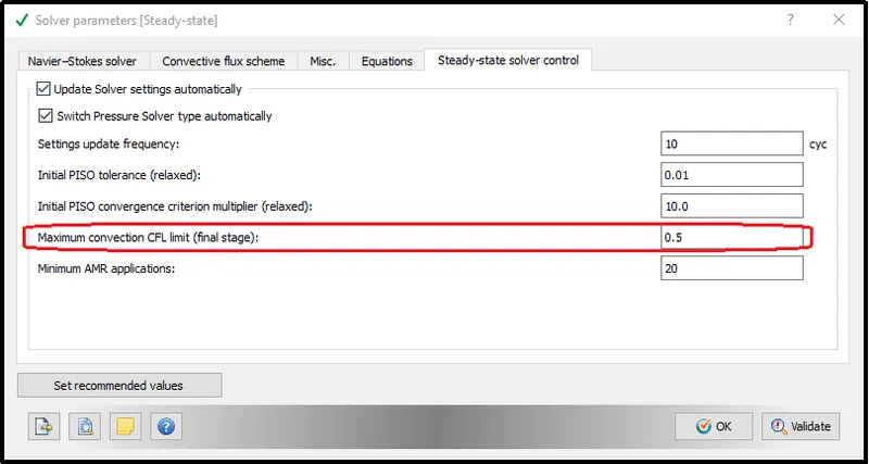
In the solver Parameter, it is very important to set Maximum convection CFL limit control below 1. For this simulation is set as 0.5

Fluid Region:-

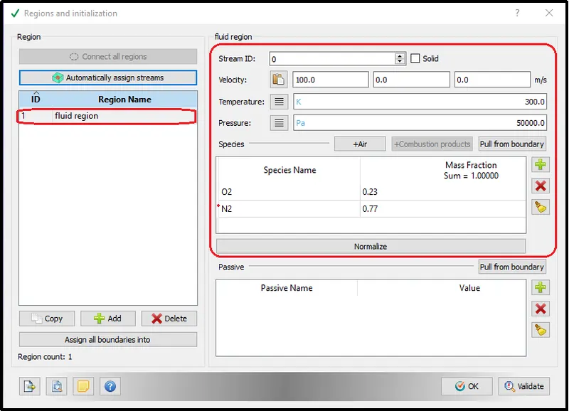
Apart from the boundary surface, cells also generate in the inner volume. Therefore, it is important to assign some material or fluid material with particular property conditions to these cells.

So, we define it as a flow region with material fluid as air with normal pressure and temperature at its initial state.

Boundary condition:-

Boundary conditions (b.c.) are constraints necessary for the solution of a boundary value problem. A boundary value problem is a differential equation (or system of differential equations) to be solved in a domain on whose boundary a set of conditions is known. It is opposed to the “initial value problem”, in which only the conditions on one extreme of the interval are known. Boundary value problems are extremely important as they model a vast amount of phenomena and applications, from solid mechanics to heat transfer, from fluid mechanics to acoustic diffusion.

Types of boundary conditions mainly used for shock wave problem in converge CFD

Both ordinary and partial differential equations need boundary conditions to be solved. Different types of boundary conditions can be imposed on the boundary of the domain. The choice of the boundary condition is fundamental for the resolution of the computational problem: a bad imposition of b.c. may lead to the divergence of the solution or the convergence to a wrong solution.

Two types of boundary conditions come across while setting up the simulation in converging CFD.

Dirichlet Boundary condition

• It is the first type of boundary condition that indicates the value of the solution on the boundary of the domain.
• The Dirichlet Boundary conditions state the value that the solution function f to the differential equation must have on the boundary of the fluid domain.
• The boundary is usually denoted as delC. Where C is the fluid domain.
• In a two dimensional domain that is described by x and y, a typical Dirichlet boundary condition would be

`f(x,y) = g(x,y,…),` where:`(x,y) in del C`

• Here the function g may not only depend on x and y, but also on additional independent variables, e.g., the time t.
• For instance, consider the example of the barrier lake used a Dirichlet boundary condition stating that the volume of the lake was 0 for t=0.
• Here the function g is constant, but it must not necessarily be the case.
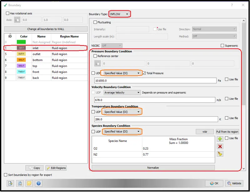
• So in this project, we are considering the inlet boundary condition as a Dirichlet boundary condition by specifying all the inlet values of pressure, velocity, and temperature.

Inlet:-

At the inlet, we are giving a Dirichlet Boundary condition of pressure 101000Pa, velocity 678m/s and Temperature 286K.

Neumann Boundary condition

• The second important type of boundary condition is the Neumann boundary conditions.
• Neumann boundary conditions state the derivative of the solution function f to the differential equation must have a given value on the boundary of the fluid domain.
• A typical Neumann boundary condition would be

`(delf(x,y))/delx = g(x,y,…)` where: `(x,y) in del C`

Or

`(delf(x,y))/dely = g(x,y,…)` where: `(x,y) in del C`

• Again the function f may not only depend on x and y, but also on additional variables such as time. We use an example of a Neumann boundary condition when deriving the velocity profile of a fluid layer on a plane driven by gravity. While solving the differential equation we state that the shear stress on the open surface of the fluid must be 0.
• This is the so-called free-surface condition. As the shear stress s calculated from the first derivative of the velocity, this is a Neumann boundary condition.

Outlet:-

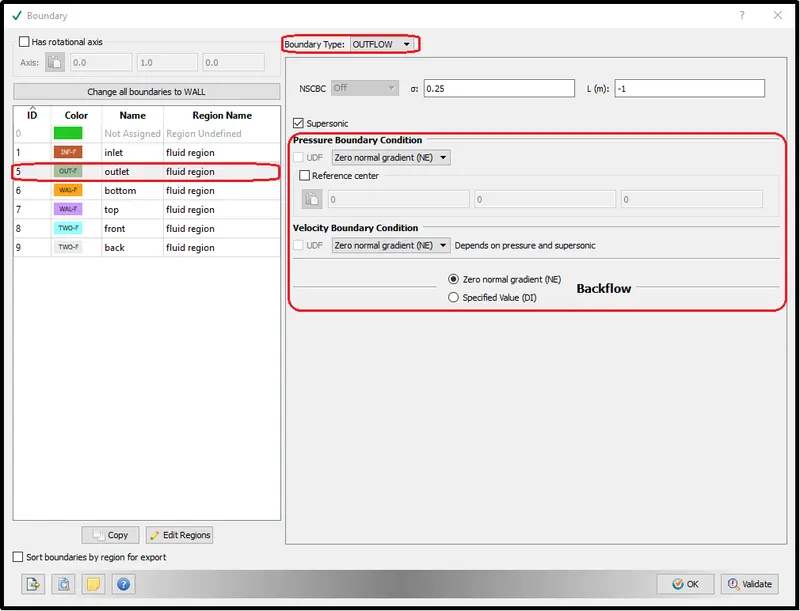
At the outlet, we are considering the Newman boundary condition where you prescribe a flux, which is the gradient of the dependent variable. Here, a zero normal gradient case is considered for pressure velocity and temperature.

Top and Bottom wall:-

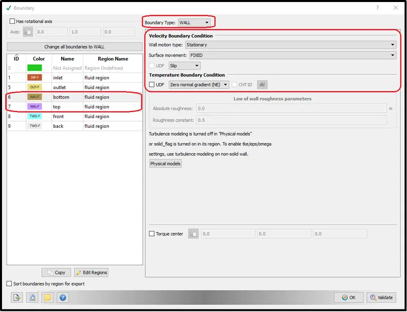
to get an expansion fan effect at the corner we have to avoid the turbulent equation effect. so that near-wall we required the slip effect so there will be no friction of the top and bottom wall.

Front and Back wall:-

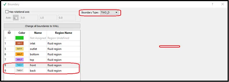
We are considering this simulation as 2D therefore the front and back surface were defined as 2D.

Grid Control/ Meshing:-

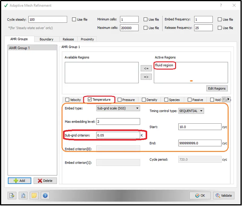
In the 'Grid Control' setting, the "Adaptive Meah Refinement" parameter was added. In which we specified the fluid region and the temperature sub-grid scale (SGS) option was selected with the max embedded level of 2.

The results were simulated for the different sub-grid scale (SGS) (for 0.05, 0.025, 0.01).

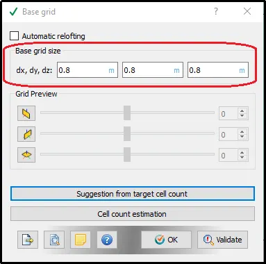
The base grid size provided is 0.8m along each direction.

Output/Post-processing:-

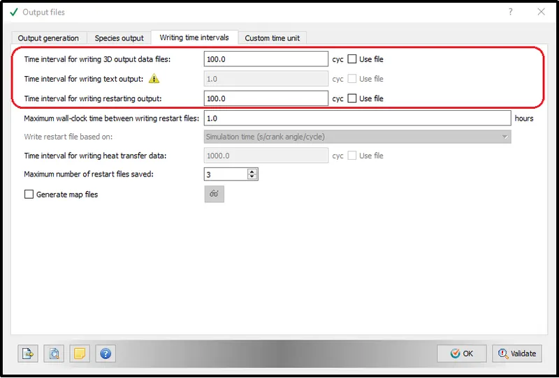
The time interval for writing 3D output data files is kept for 100 cycles i.e. after 100 cycles it will create one 3D output file.

The time interval for writing restarting output was also kept for 100 cycles which will help us restart the simulation in the last count of 100 cycles in case simulation stopped unexpectedly. It helps to save the simulation time of the user.

Output Results:-

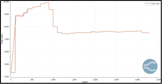
SGS temperature value = 0.05(Velocity 678m/s)

Total Cell variation throughout the complete simulation

Velocity, Pressure, Temperature and Density animation:-

In the below animations, the first upper left side animation shows velocity contour, the second animation mounted on the upper right side depicts the pressure variation, the third lower left animation shows the Temperature variation and the final lower right animation shows the density variation.

Here, we can notice the near the corner or shape area the mesh resolution starts to increase because of the effect of the SGS temperature value. The expansion fan is generated because of mach number more than 1 which is, in this case, the velocity of 678m/s - 1.97 mach number.

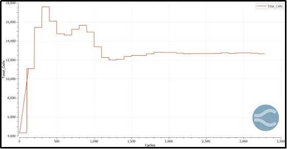
SGS temperature value = 0.025(Velocity 678m/s)

Total Cell variation throughout the complete simulation

Velocity, Pressure, Temperature and Density animation:-

As we provide the lower SGS temperature value, we can observe more fine mesh as compare to earlier animation.

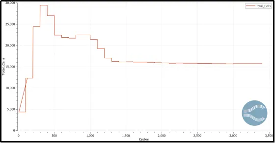
SGS temperature value = 0.01(Velocity 678m/s)

Total Cell variation throughout the complete simulation

Velocity, Pressure, Temperature and Density animation:-

• If we again provide a lower value of SGS temperature as 0.01 the finer the mesh becomes near the corner or sharp edge, near the starting angle of the expansion fan.
• The physical meaning of sub-grid temperature is an error between the actual temperature and resolved temperature at each cell. Converge calculates this value as its simulation.
• If this error is larger than the user-specified value, Converge refines the cell automatically. There is a time if the total cell count has already reached the maximum cells. The cell refinement operation will NOT proceed.
• If the error is smaller than 20% of the user-specified value, embedding on this cell will be released. By giving different user-specified values, the results can change as the error introduced to the simulations system varies.
• Reducing the temperature SGS size minimizes the error and improves the resolution of the contour plot animation.

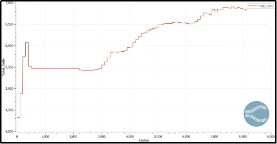
SGS temperature value = 0.05 (Velocity 100m/s)

Total Cell variation throughout the complete simulation

Velocity, Pressure, Temperature and Density animation:-

To observe how our solution will look the setup was simulated using 100m/s - 0.292 mach number. which do not shows the efficient expansion fan effect near the sharp edge.

Conclusion:-

• Shock-turbulent interactions are a common occurrence in the supersonic flow because the compression and flow deflection is almost always accompanied by the formation of a shock.
• The characteristics of the interaction depend on the Mach number, the nature of the incoming flow, the shock angle, the source of the shock, and the flow geometry.
• Dirichlet condition specifies the value that the unknown function needs to take on along the boundary of the domain.
• Neumann boundary condition specifies the values that derivatives of a solution are going to take on the boundary of the fluid domain after imposing an ordinary (ODE) or partial differential equation (PDE).
• If we again provide a lower value of SGS temperature, the finer the mesh becomes near the corner or sharp edge, near the starting angle of the expansion fan.

References:-

[1] Prandtl-Meyer Angle - https://www.grc.nasa.gov/www/k-12/airplane/pranmyer.html

[2] Evaluating Oblique Shock Waves Characteristics on a Double-Wedge Airfoil - Evaluating Oblique Shock Waves Characteristics on a Double-Wedge Airfoil (scirp.org)

[3] Shock Wave-boundary layer Interactions - https://link.springer.com/chapter/10.1007%2F0-387-26305-5_10

[4] Types of Boundary conditions:- https://www.sciencedirect.com/topics/engineering/dirichlet-boundary-condition