Week 5: Prandtl Meyer Shock problem

Aim: To simulate the prandtl Mayer shock flow in converge CFD

1. Shock flow boundary conditions.

Do a literature search on what BC's are typically used for shock flow problems.

2. What is a shock wave?

In your own words, describe the physics behind shock waves.

3. Effect of SGS parameter on shock location.

In the Prandtl Meyer shock problem, look at the effect of SGS temperature value on cell count and the shock location.

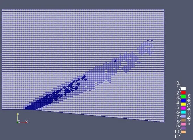
4. It is expected to show the mesh generation using PARAVIEW.

5. And also create an animations.

1. Shock flow boundary conditions:

Boundary conditions play an important role for solving any kind of problem. Basically appropriate boundary conditions are needed for solving the steady state flow problem. It is one of the basic requirement of the mathematical model. On the other hand, for solving the transient flow problem, appropriate initial conditions are required.

Boundary conditions are of generally three types

• Dirichlet boundary condition
• Neumann boundary condition
• Robin type boundary condition

In Dirichlet boundary condition the value of the function is specified at the boundary.

In Neumann boundary conditon, the value of the normal derivative of a function is specifeid.

Robin type boundary condition is the combination of both Dirichlet and Neumann boundary condition.

Why is Neumann boundary condition used for supersonic outlets?

Because the values of all the variables (pressure, velocity, temperature, Mach no) are not available before solving the problem. So nothing is specifed at the supersonic outlet and all the variables are extrapolated from the domain interior. Only the Normal derivative (Normal with respect to the outlet boundary) of variables are specified as 0 (zero gradient).

However, if any pressure and velocity value is specifed at the outlet the solution will not converge and become unstable.

2. What is a shock wave?

In physics, a shock wave (also spelled shockwave), or shock, is a type of propagating disturbance that moves faster than the local speed of sound in the medium. Like an ordinary wave, a shock wave carries energy and can propagate through a medium but is characterized by an abrupt, nearly discontinuous, change in pressure, temperaure and density of the medium.

For the purpose of comparison, in supersonic flows, additional increased expansion may be achieved through an expansion fan, also known as a prandtl-Mayer expansion fan. The accompanying expansion wave may approach and eventually collide and recombine with the shock wave, creating a process of destructive interference. The sonic boom associated with the passage of a supersonic aircraft is a type of sound wave produced by constructive interference.

Unlike solitons (another kind of nonlinear wave), the energy and speed of a shock wave alone dissipates relatively quickly with distance. When a shock wave passes through matter, energy is preserved but entropy increases. This change in the matter's properties manifests itself as a decrease in the energy which can be extracted as work, and as a drag force on supersonic objects; shock waves are strongly.

Shock waves can be:

Normal

At 90° (perpendicular) to the shock medium's flow direction.

Oblique

At an angle to the direction of flow.

Bow

Occurs upstream of the front (bow) of a blunt object when the upstream flow velocity exceeds Mach 1.

Some other terms:

• Shock front: The boundary over which the physical conditions undergo an abrupt change because of a shock wave.
• Contact front: In a shock wave caused by a driver gas (for example the "impact" of a high explosive on the surrounding air), the boundary between the driver (explosive products) and the driven (air) gases. The Contact Front trails the Shock Front.

Prandtl Mayer Shock

A supersonic expansion fan, technically known as Prandtl–Meyer expansion fan, a two-dimensional simple wave, is a centered expansion process that occurs when a supersonic flow turns around a convex corner. The fan consists of an infinite number of Mach waves, diverging from a sharp corner. When a flow turns around a smooth and circular corner, these waves can be extended backwards to meet at a point.

Each wave in the expansion fan turns the flow gradually (in small steps). It is physically impossible for the flow to turn through a single "shock" wave because this would violate the second law of thermodynamics.

Across the expansion fan, the flow accelerates (velocity increases) and the Mach number increases, while the static pressure, temperature and density decrease. Since the process is isentropic , the stagnation properties (e.g. the total pressure and total temperature) remain constant across the fan.

The theory was described by Theodor Mayer on his thesis dissertation in 1908, along with his advisor Ludwig prandtl , who had already discussed the problem a year before.

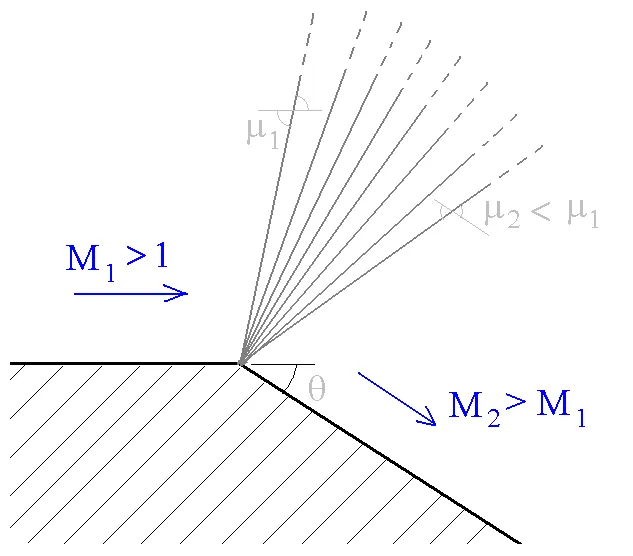
When a supersonic flow encounters a convex corner, it forms an expansion fan, which consists of an infinite number of expansion waves centred at the corner. The above figure shows one such ideal expansion fan.

The expansion fan consists of an infinite number of expansion waves or Mach lines. The first Mach line is at an angle `mu_1 = arcsin(frac(1)(M_1))` with respect to the flow direction, and the last Mach line is at an angle `mu_2 = arcsin(frac(1)(M_2))` with respect to final flow direction. Since the flow turns in small angles and the changes across each expansion wave are small, the whole process is isentropic. This simplifies the calculations of the flow properties significantly. Since the flow is isentropic, the stagnation properties like stagnation pressure `P_0`,stagnation temperature `T_0` and stagnation density (`rho_0`) remain constant.

3. Effect of SGS parameter on shock location.

Use Adaptive Mesh Refinement (AMR) to automatically refine the grid based on fluctuating and moving conditions such as temperature or velocity. This feature may be used to obtain a refined grid in flow regions of interest allowing complex phenomena, such as flame propagation or high-velocity flow, without unnecessarily slowing the simulation with a globally refined grid.

There are two types of AMR: sub-grid scale (SGS)-based and value-based. The AMR type and criteria should be chosen such that a higher grid resolution (embedding) is added where the flow field is most under-resolved, where the sub-grid field is the largest (i.e., where the curvature [gradient] of a specified field variable is the highest), or where a variable satisfies
the embed criteria. The default AMR method in CONVERGE estimates the magnitude of the sub-grid field to determine where CONVERGE will add embedding.

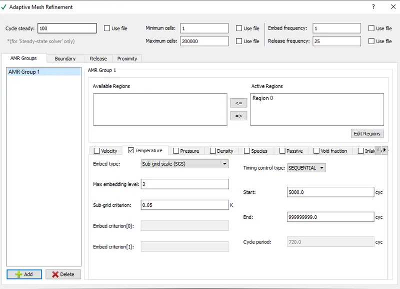
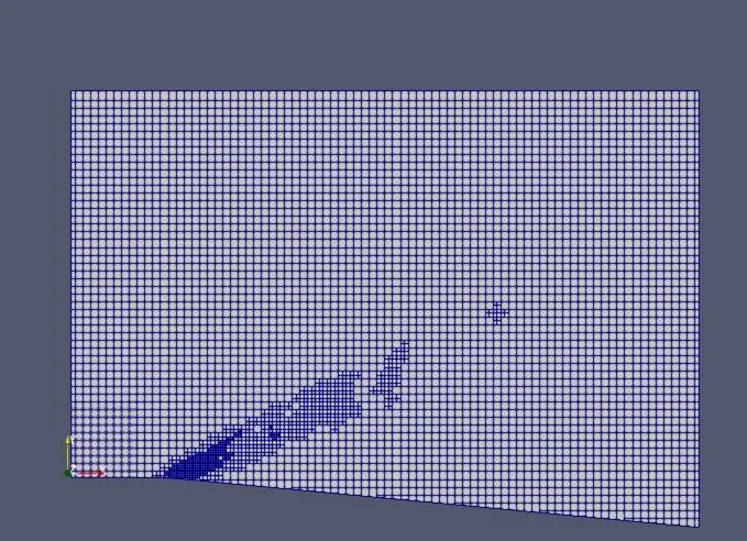
Adaptive mesh refinement technique was used because the region where shock would occur require the mesh to be refined locally. The mesh in the other regions have the same size as the base grid size whereas the region where shock occurs finer cells are used. Temperature based mesh refinement was used that would monitor curvature in temperature. Temperature based mesh refinement was used that would monitor gradient in temperature. Gradient means `frac{partial^2t}{partialx^2}`. When temperature is greater than a particular value defined by the user the mesh is refined. In the first run, the SGS is taken as 0.05K. When subgrid is greater than 0.05K, the mesh would refine.

Geometry preparations

• Open the new project and load the stl file of geometry.

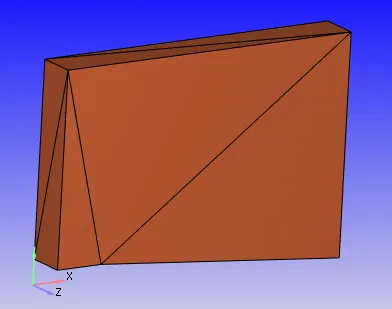
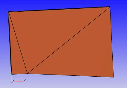
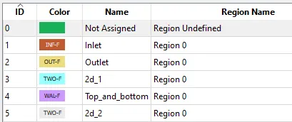
• Add the boundaries by clicking create multiple boubdaries to create all boundaries at a once and name them like Inlet, Outlet, Top, bottom, 2d_1(front) and 2d_2(back) by selecting the respective triangles.

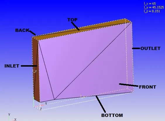
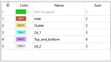
• Then click Normal Toggle option and click any one of the triangle which shows the normal that is opposite to the direction of fluid flow and click Apply.
• To ensure that the geometry is clean, click Diagnosis tab and click on Find.
• All the parameters that got checked shows the green colour tick mark.
• Case-setup
• In order to begin the case-setup, click on the case-setup and click begin case-setup and click Time based, since it is not a crank angle based like IC engines or Pumps but a steady-state channel flow setup.
• Then click on Materials and select Air to be predefined mixtures.
• Then open the Gas simulation and Global transport parameters and retain the default setting. And also retain the same setting for the species and Reaction mechanism.
• Then click on the Run Parameter under the Simulation Parameter and choose the transient solver under the solver tab and then choose the Full Hydrodynmic under the simulation mode. And then choose the Compressible under the Gas flow solver.
• In the Miscellaneous tab, check the steady state monitor and uncheck the use shared memory because of we are running a steady state simulation flow here.
• Then click on the Steady-state monitor, click add config. And click Add to add the variables that needs to be monitored.

• 

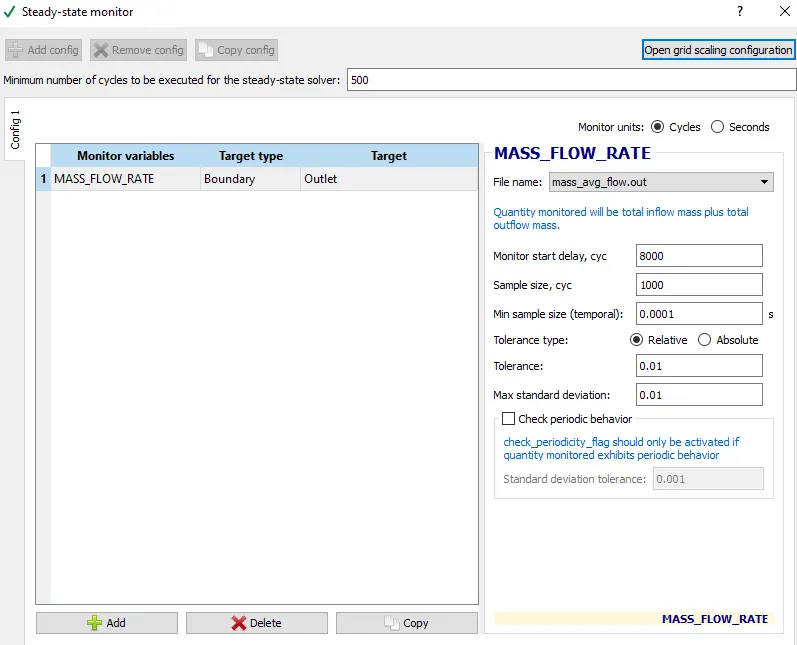
  • The monitor start display is a parameter that ensures that the simulaion runs for a certain number of cycles before the variable can be monitored. This is especially useful in transient simulations when you want the solution to run for a particular amount of time before checking for convergence, if the steady state results are also required.
  • Sample size denotes the number of cycles or seconds over which the variable is checked to see if the solution has converged. The solution is said to be converge when the average change over multiples iterations is less than the tolerance value. The tolerance value can be changed based on the problem and level of accuracy required.
  • In the simulation time parameter do the following changes.

  

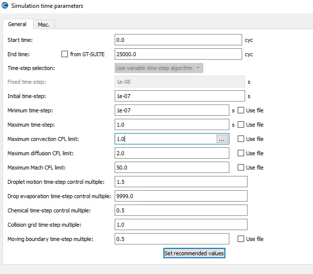
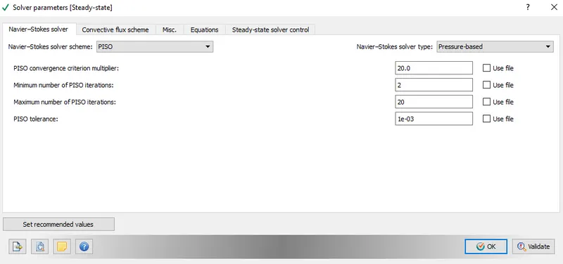
  • In the solver time parameter, we only choose the pressure based solver and retain the remaining setting.

  

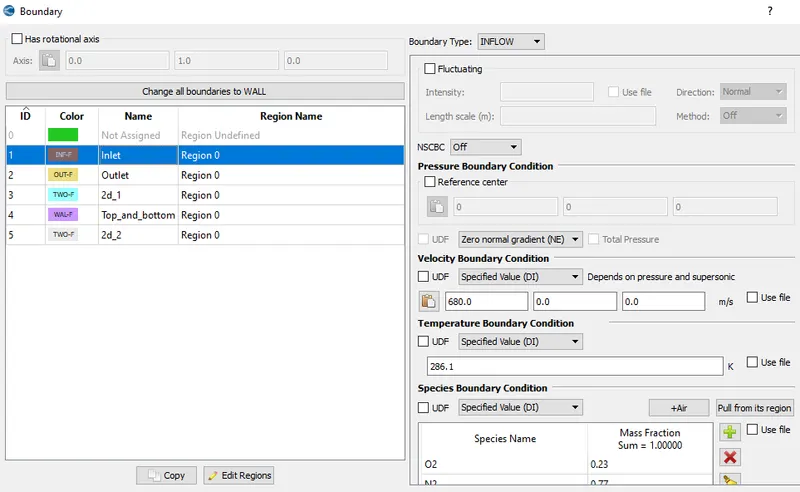
  • At the inlet boundary we specify the velocity 680 m/s and select the predefined mixture as a Air which contains N2 as a 77% and O2 as 23%. And select the temperature to be specified of 286.1K. And we are taking the zero normal gradient(NE) for the pressure boundary condition at the inlet.

  

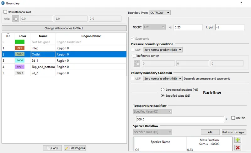
  • At the outlet boundary, we specify the zero normal gradient boundary condition for both pressure and velocity. And give the temperature 300K at the outlet boundary.

  

  • At the front and back wall, we are specify the 2d boundary condition.
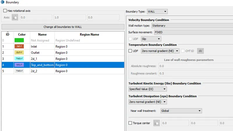
  • At the top and bottom wall, we are taking the slip boundary condition.

  

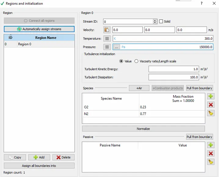
  • In Regions and Initializations, click Add as Region 0.

  

  • Goto Physical Models and check the Turbulence Modelling and choose the RNG/k-epsilon model.
  • Then in the grid control, the mesh size that want to be created is in meters.

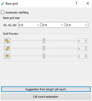
The adaptive mesh refinement is a method of adopting the accuracy of the solution within a certain sensitive or turbulent region of simulation, dynamically and during the time the solution is being calculated. When curvature exceeds a particular value, the cell will be embedded.

we used this formula for the AMR

Size of the cell in scaled grid = (Size of cell in base grid) / 2^(amr_embed_temp_scale)

for exmple

Base grid = 0.8m

amr_embed_temp_scale = 2

size of cell in base grid = 0.8/2^2 =0.8/4=0.2m

Then the temperature based AMR will be done as

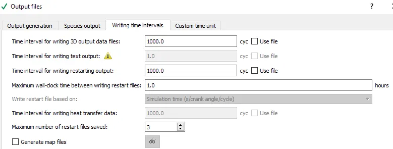
• For Output files, Time inter for writing 3D output files is 100 cycles which is the time interval between the one and another output file that get dumped in output files successively and the maximum no. of restart files that saved is 3 which is a factor of safety and click ok.

• 

  • Now when we click on validate all options for validating, we got the errors.
  • To Resolve these errors, we go to Regions and initializations and rename the region 0 to Voulmetric region user defined and then go Boundary to assign this region to all the boundaries we have ceated since the error is not assigning the region for those.

  

  • And then click on validate all again and there will be no errors and the validation has been successfully complete.
  • At the end all the inputs files have to be exported:

  File -->Export-->Export input files

The simulation was run under three different SGS criterian and also for subsonic fow velocity is taken 100 m/s.

1. SGS = 0.05K
2. SGS = 0.01K
3. SGA = 0.1K
4. Subsonic flow = 100 m/s

   Mesh

• SGS = 0.05K

S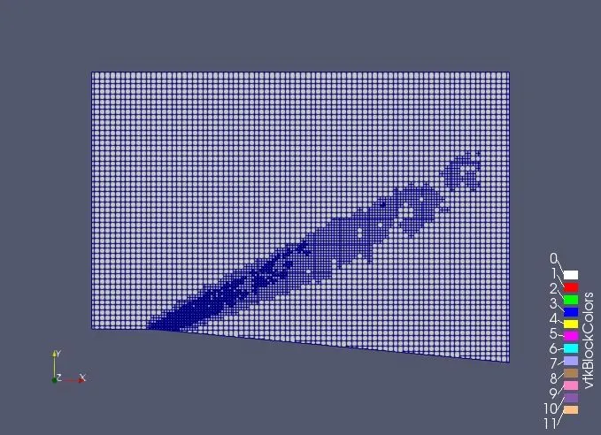

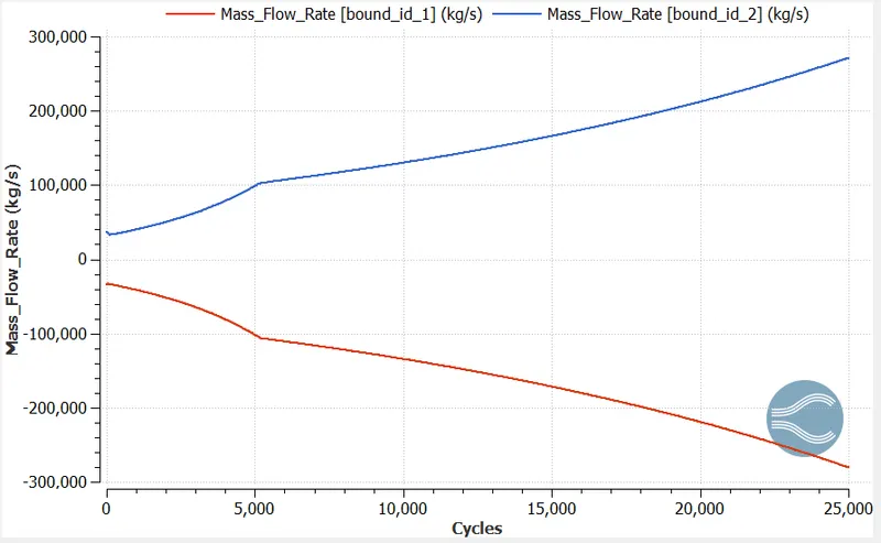
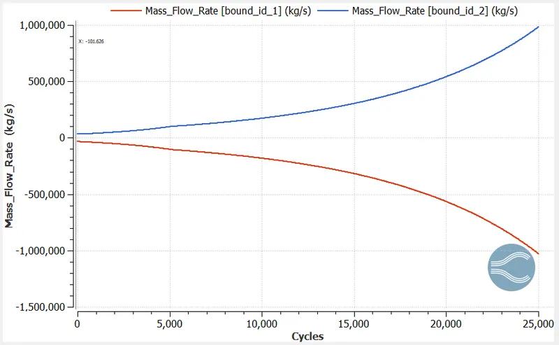
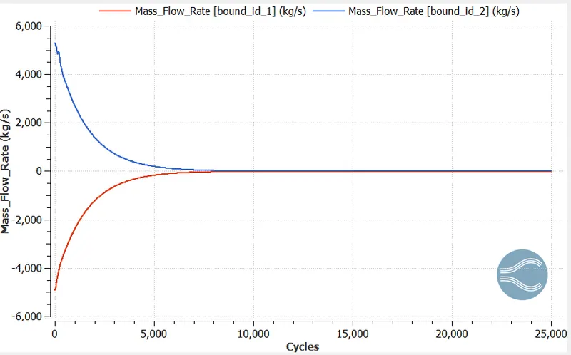
Mass Flow Rate

Mass_Flow_Rate [bound_id_1] = Inlet

Mass_Flow_Rate [bound_id_2] = Outlet

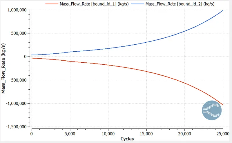
• Mass flow rate is defined as the mass of substance which passes per unit time.
• Here the mass flow rate at the inlet is decreased due to high pressure and low velocity and after 5000 cycles the mass flow rate is gradually decreases.
• Then Finally at the inlet the value of the mass flow rate is -1,000,000 (kg/s) and at the outlet the value of mass flow rate is 1,000,000 (kg/s).
• At the inlet negative sign shows that the mass is going to inside and the outlet positive sign shows that the mass is going to outside.

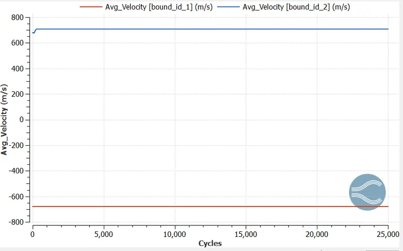
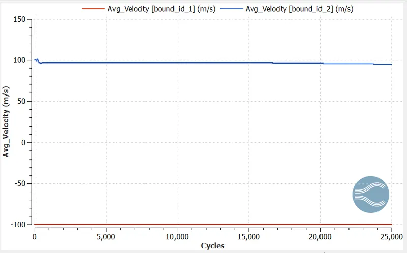
Avg Velocity

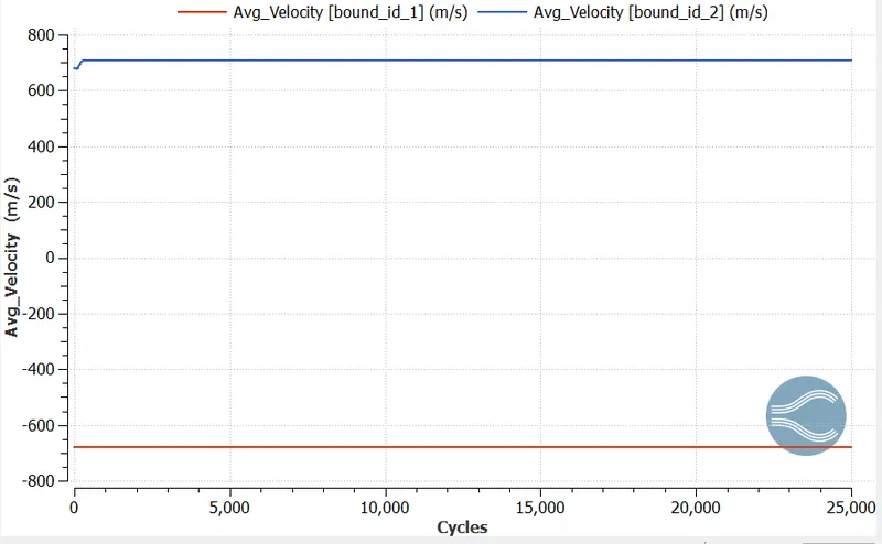
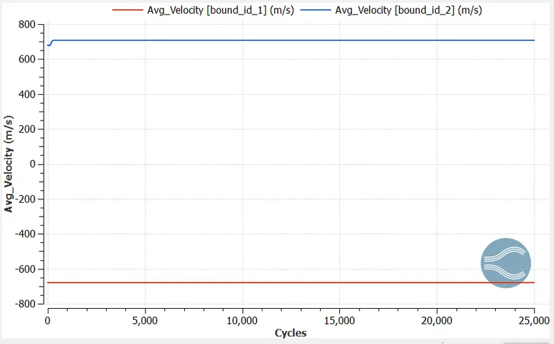
• In the above velocity plot, we easily observe that at the inlet velocity is gradually decreases due to increase in pressure at inlet
• At the outlet, we observe that the velocity is gradually increasing due decrease in pressure.
• At inlet the velocity is decreased and reaches to -150 m/s and at the outlet the velocity is increased and reaches to 53 m/s.
• It occurs since the pressure is inversely proportional to the velocity.

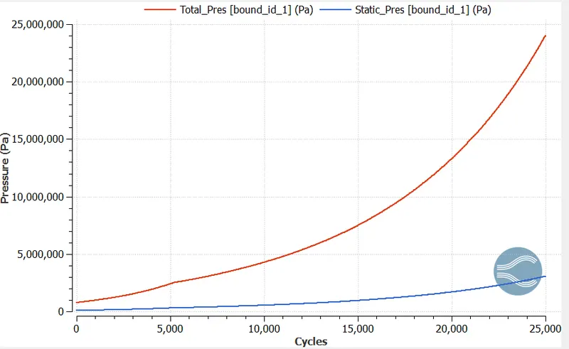
Pressure

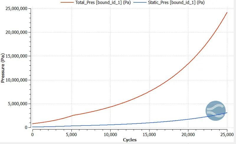
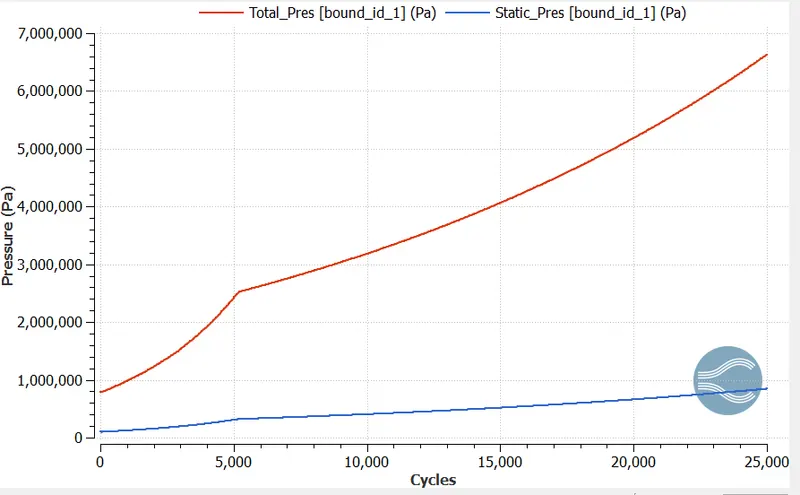
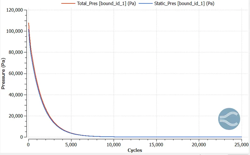
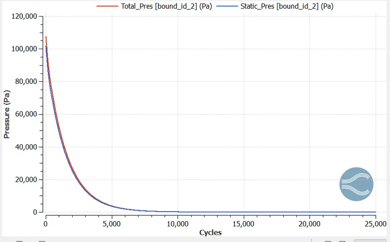
• At the inlet plot of pressure, we observe that initially total and static pressure is same which is 110,310Pa. And we also know that total pressure = static pressure+dynamic pressure and initially dynamic pressure is zero.
• As the cycles going on the static pressure is going to decrease due to increase in dynamic pressure.
• After 1500 cycles the static pressure is going to decrease rapidly due to fastly movement of fluid.

Mach Number

Formula of Mach no is

`M = frac{u}{c}`

Where u is the local flow velocity and c is the speed of sound.

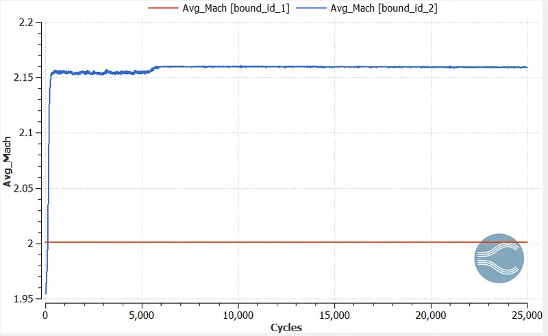
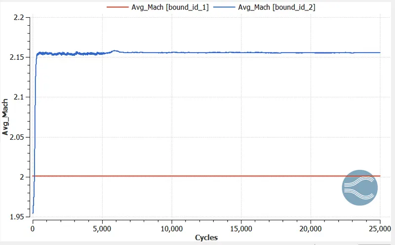
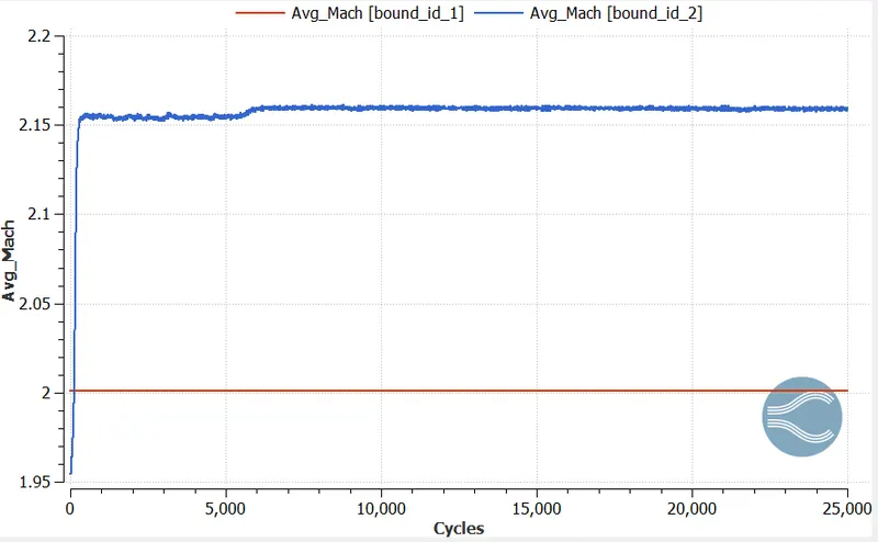
In this case we are taken, the velocity along the x-axis is 680 m/s and roughly the speed of sound is taken 340. So the inlet mach no is 2.0 approximately.

In the avove graph we observe that at the inlet mach no is 2 and there ia an increase in mach no at outlet. Across the expansion fan the flow accelerates and then Mach number increases. At the outlet the value of mach number is 2.15. As there is shock occuring that's why increase in velocity and also increase in Mach number happening.

Total Cells

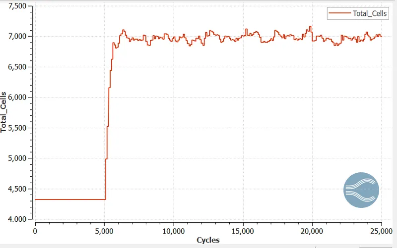
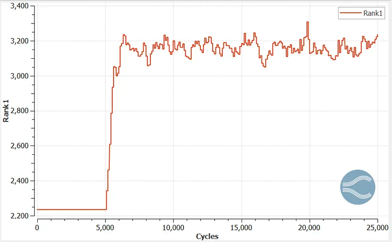
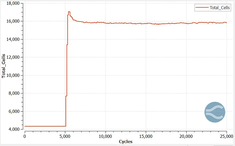
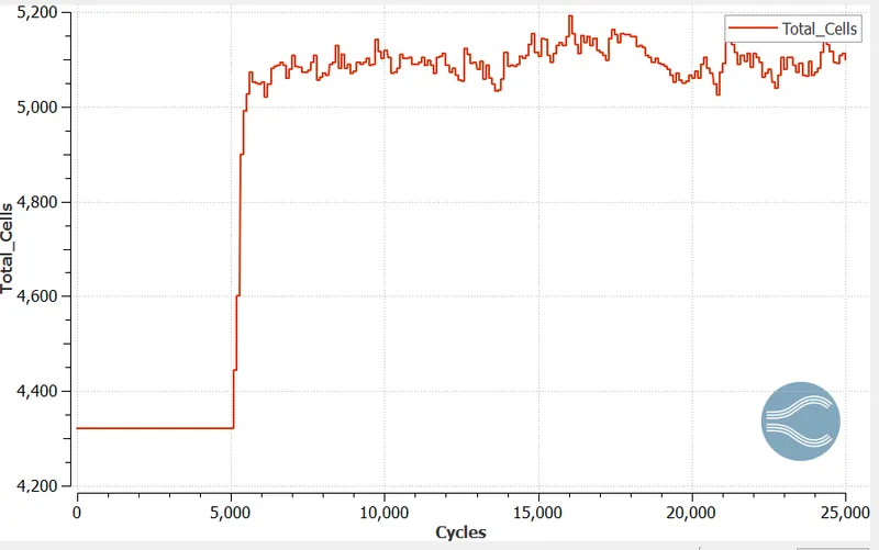
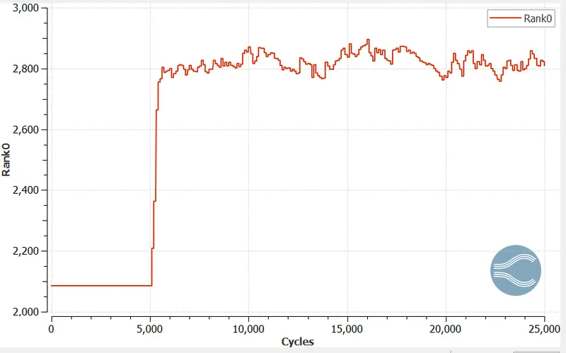
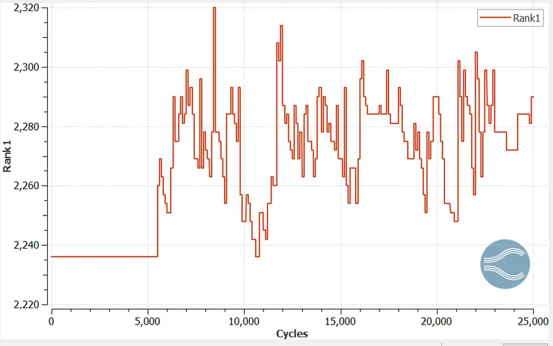
Above graph represent the total no of cells which is approximately 7,000. As we did in the above setting that the adaptive mesh refinement is start after 5,000 and that's why there is an sudden increase occur in the no of cells. Because after 5,000 iterations mesh is going to refine and also the capturing of shock wave are also started here.

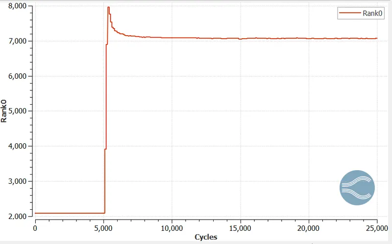
Rank_0

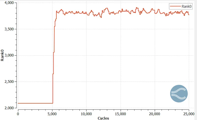
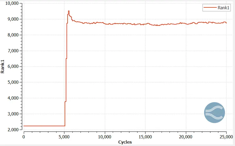
Rank_1

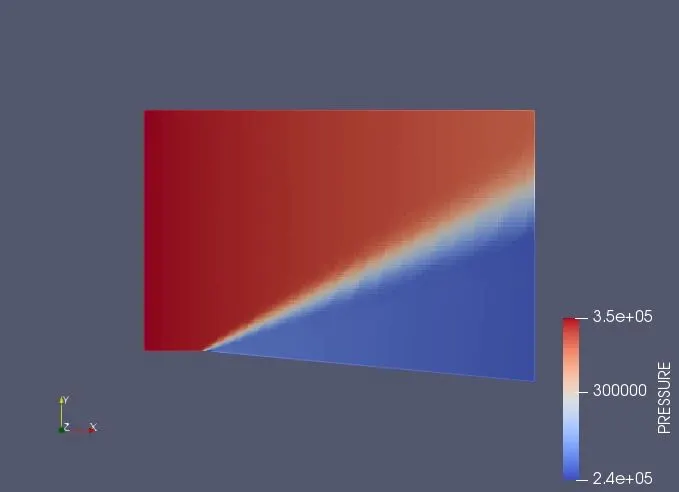
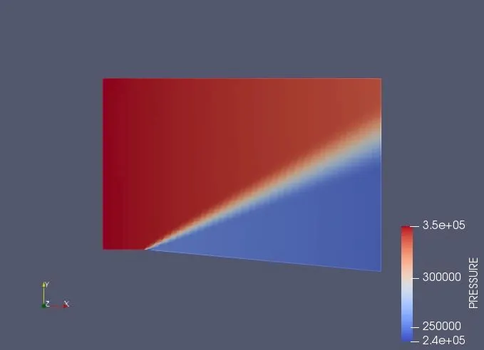
Pressure Contours

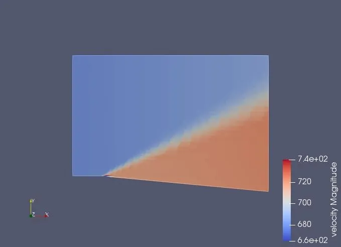
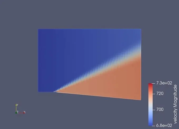
Velocity Contours

Velocity animation

Pressure animation

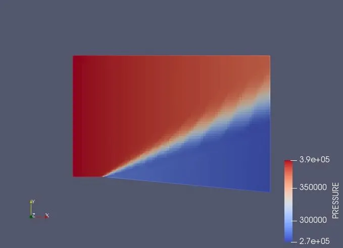
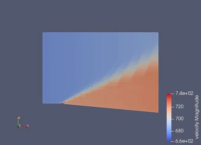
In the above velocity and temperature contours we can easily observe that the AMR has ben captured. AMR we are using here is the temperature based. Whenever curvature value `frac{d^2T}{dx^2}`exceed a particular value, cells will be embedded.

• SGS = 0.01K

Mesh

Mass flow rate

Pressure

Avg Velocity

Avg Mach number

Total Cells

Rank_0

Rank_1

Pressure Contours

Velocity Contours

Pressure animation

Velocity animation

SGS 0.1

Mesh

Mass flow rate

Avg Veocity

Pressure

Avg Mach no

Total_cells

Rank-0

Rank_1

Pressure contours

Velocity contours

Velocity animation

Pressure animation

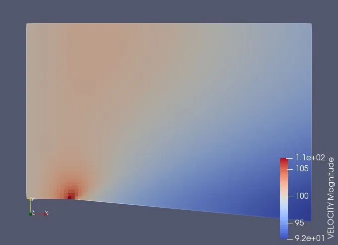
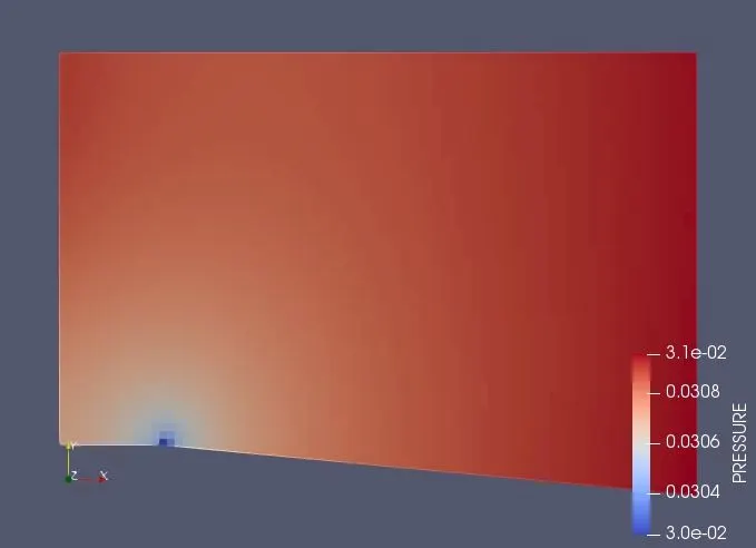
100 m/s Velocity and SGS= 0.1 Results

Mesh

Mass flow rate

Velocity

Pressure

Mach no

Cell Count

Velocity contours

Pressure Contours

Pressure animation

Velocity animtion

Conclusion

• We are successfully simulating the supersonic and subsonic prandtl flow in a 2D duct having a sharp corner was setup and run in converge CFD. Various contours plots of velocity, pressure, density and temperature were studied.
• We ran the simulation at different SGS values and concluded the results.
• We also run the simulation using the velocity 680 m/s and 100 m/s.
• Changing the SGS values changes the number of cells that are formed during meshing. As mentioned above when Sub-grid temperature is greater than SGS value, the mesh is refined.
• For the low value of SGS(0.01 and 0.050 more cells are refined than the higher value of SGS(0.1).
• The inlet Mach no where flow enter to the geometry is 2 and the outlet mach no is 2.15 which correspond to an outlet velocity 732m/s as compared to the inlet velocity 680m/s.

Effect of SGS parameter on shock location and total cell count

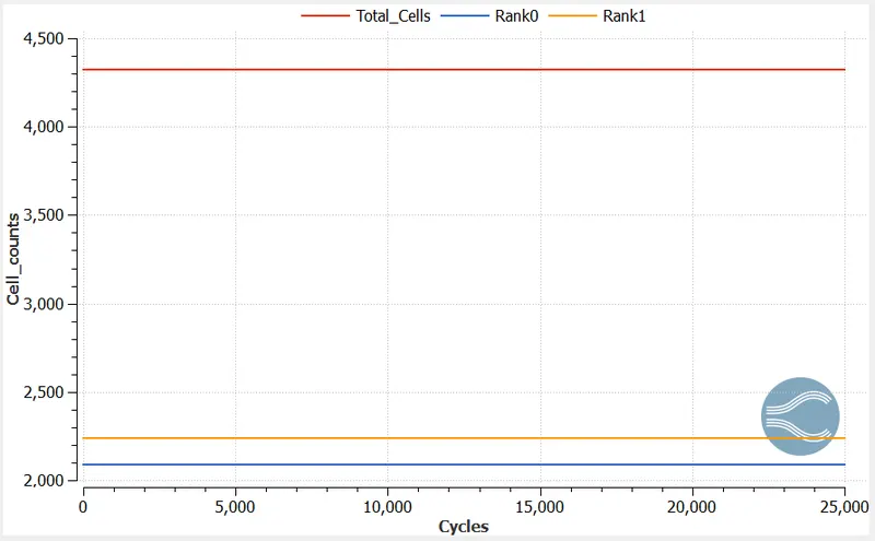
Cell Count: As the SGS parameter decreases, the total cell count increases. In other words, for small SGS parameter AMR refines the mesh for more number of cells in and around the shock wave.

Shock Location: For high SGS parameter, the mesh refinement area is very small like (SGS = 0.1) and for the small SGS parameter, the mesh refinement area spans from the sharp edge till the outlet boundary.

Subsonic Vs Supersonic flow comparison

In supersonic flow, the prandtl mayer expansion fan is clearly visible and the mesh refinement is also in the shock region. Whereas on the other hand , in the case of subsonic flow, the prandtl mayer shock fan is not clearly visible and even the mesh refnement is not visible. This is because there are no sudden fluctuations in pressure, velocity, temperature or density or in other words shock.

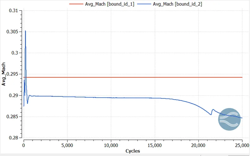
Also the average Mach number inceases from the inlet to the outlet in case of supersonic flow and deceases in case of subsonic flow.