Prandtl Meyer Shock problem
Aim: To perform a steady state simulation on given Prandtl-Mayer expansion fan model and discuss the results.
Objective:
1) To discuss about the boundary conditions used for shock flow problems.
2) To discuss the physics behind the shock waves.
3) To observe and discuss the effects of SGS temperature value on cell count and shock location.
- Case 1- perform steady state simulation for supersonic flow for sub grid scale = 0.05
- Case 2- perform steady state simulation for supersonic flow for sub grid scale = 0.03
- Case 3- perform steady state simulation for subsonic flow for sub grid scale = 0.05
Introduction:
Shock wave
In physics, a shock wave is a type of propagating disturbance that moves faster than the local speed of sound in the medium. The shock wave carries energy and can propagate through medium but is characterized with an abrupt, nearly discountinuous, change in pressure, temperature and density of the medium. The below figure describes the flow behaviour.
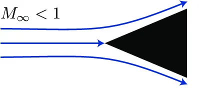
(a) subsonic flow
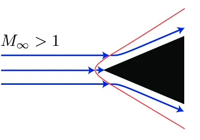
(b) supersonic flow
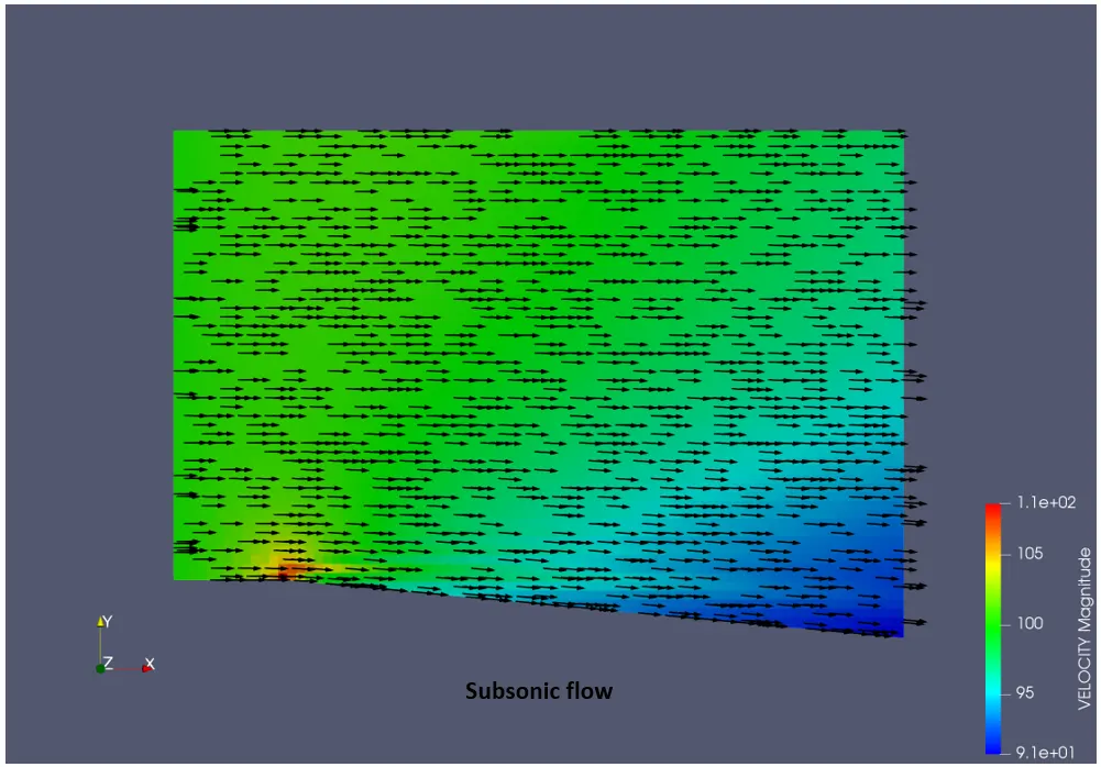
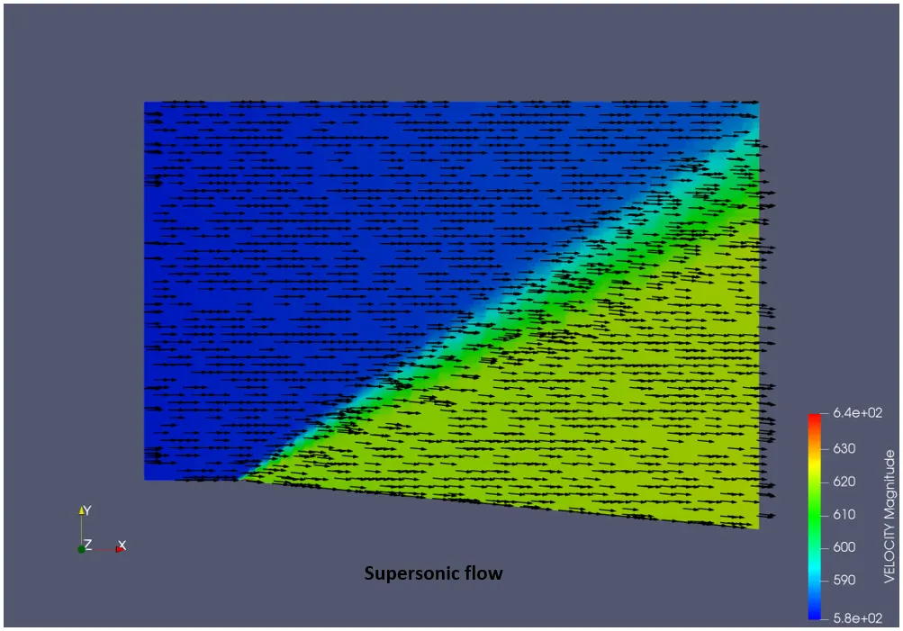
To understand the physics about the formation of shock waves, consider a triangular block placed in a flow as shown in Fig. (a) and Fig. (b). The kinetic theory tells that the flow consists of a large number of fluid molecules in unit volume and transport of mass, momentum and energy takes place through the motion of these molecules. The molecules carry signals generated by the disurbance caused by the presence of obstacles, these signals are generated when the flow field around the obstacle is equal to or less than speed of sound. In Fig. (a), the incoming fluid stream is subsonic and the molecules far upstream of the triangular block get the information about the presence of the obstacle through the signal in advance before reaching the block. Therefore, the molecules in the fluid orient themselves in order to flow around the triangular block. In Fig. (b), the incoming fluid stream is supersonic which is greater than the spees of the sound, hence the molecules travel faster than the sound wave signals, and due to this the molecules do not get the information about the presence of the obstacle which further causes the reflected signals to coalesce at a short distance ahead of the obstacle. This coalescence forms a thin compression front called shock wave.
Prandtl-Mayer expansion fan
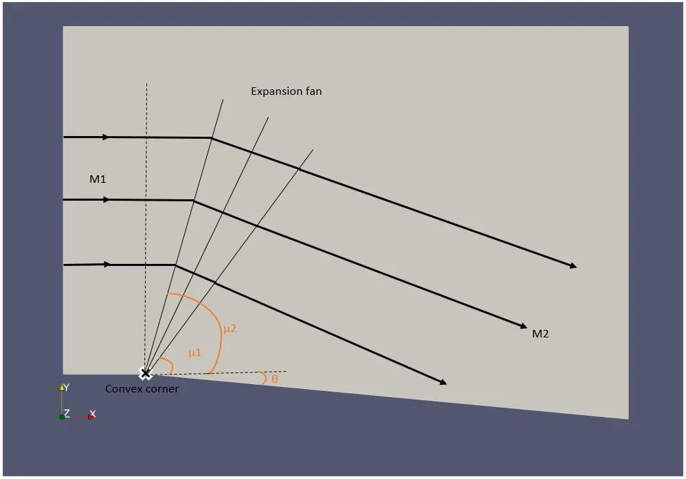
The above figure shows the convex corner and Prandtl-Mayer fan and mach lines and mach angle. The lines at which the pressure disturbance is concentrated is known as 'mach lines' and the angle between the mach line and direction of fluid flow is known as 'mach angle'. The point at which pressure disturbances are concentrated is known as 'convex corner'. In the prandtl-mayer expansion fan, there are two mach lines, one at an angle mu1 to the initial flow direction and the other at an angle mu2 to the final flow direction. The change in mach number from M1 to M2 takes place through an infinite number of mach waves.
In this simulation, the turning of a two-dimensional supersonic flow and subsonic flow through a finite angle at a convex corner which is also known as prandtl-mayer expansion fan is studied.
Boundary conditions used for shock wave problems
There are usually two types of boundary conditions which is often used in the CFD.
1. Dirichlet boundary condition
In this type of boundary condition, the solution value that the partial differential equations must have is specified at the boundary. In other words, the dirichlet boundary condition is used when the parameters at a particular boundary is known and the parameters at the other boundary is to be found. In this simulation, the fluid velocity value at inlet is specified to calculate other variables.
2. Neumann boundary condition
In this type of boundary condition, the derivative of the solution value that the partial differential equations must have is specied at the boundary. This specified derivative or the first derivative of the solution is used to calculate the desired variables at other boundaries. In this simulation, the pressure values at inlet and outlet is specified as zero gradient and is calculated from the first derivative value.
The cauchy boundary condition, mixed boundary condition and robin boundary condition are all different types of combination of Dirichlet and Neumann boundary condition.
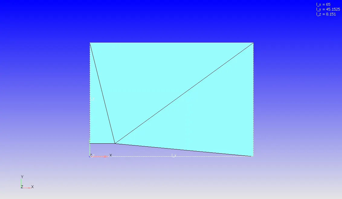
Geometric model of the Prandtl-Mayer expansion fan
Boundary conditions
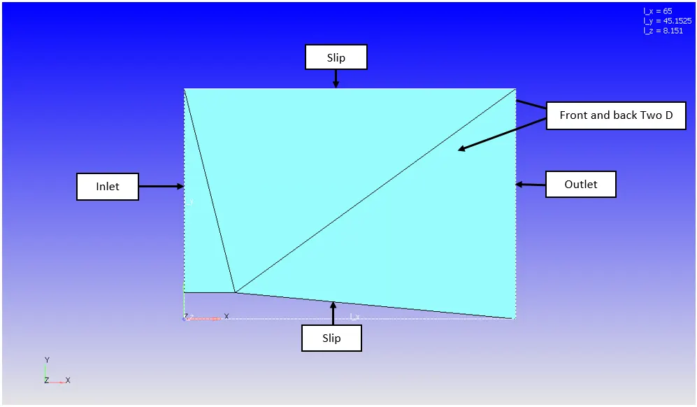
Inlet
Boundary type = inflow
Inlet velocity values for different cases

Pressure = Zero gradient (NE)
Temperature 286.1 K
Species = air
Outlet
= Outflow
velocity = zero gradient (NE)
Pressure = zero gradient (NE)
Temperature = 300 K
Species = air
Top and bottom surface
Boundary type = Wall with slip boundary condition
Front and back surface
Boudnary type = Two-D
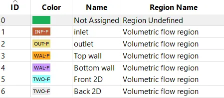
Assigning volumetric fluid region to all the bounaries
Solver type = Density based steady state solver
Solver scheme = PISO
Simulation time parameters
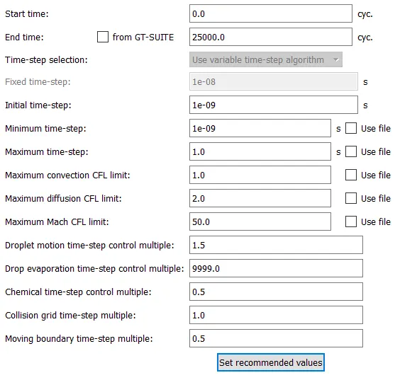
The geometry and case remains same for both the cases except for the sub grid scale, whose effects on shock location is studied. The boundaries are flagged to the respective regions and air is added as the volumetric fluid region. The velocity of the fluid from inlet is 680 m/s which is supersonic flow for case 1, case 2 and for case 3 the velocity of fluid from inlet is 100 m/s which is subsonic, and the pressure at inlet and outlet is set to zero gradient which is calculated by the nueman boundary condition. The top and bottom wall is treated as slip boundaries, where the velocity profiles do not have zero values with respect to the surface at the point of contact between the fluid and solid surface. The steady state density based solver is used, as the fluid is compressible.
The mesh is generated and refined with the help of adaptive mesh refinement. The simulation consists of three cases (case 1, case 2 and case 3), where in each case the mesh size is changed by sub-grid-scale. In order to refine mesh in the regions where shock flow occurs, the adaptive mesh refinement based on temperature is used for mesh refinement. In the adaptive mesh refinement method, the mesh is refined based on the subgrid temperature value and number of embedding layers. In other words, the mesh is refined in the regions where the subgrid temperature is greater than the specified temperature. The number of embedding layers and base grid size defines the size of the cells. The size of cells in the scaled grid is given by the formula,
(size of cells in base)/2^(max number of embedding layers)
The mesh generated and results obtained for each case is discussed below.
Case 1 (supersonic flow)
Grid control
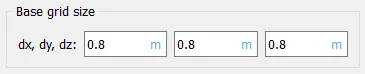
Adaptive mesh refinement
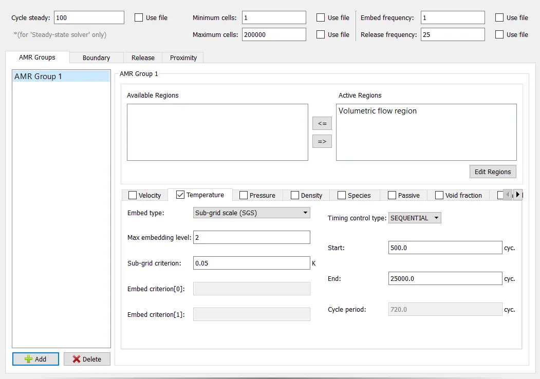
Mesh generated for SGS = 0.05 k
Results
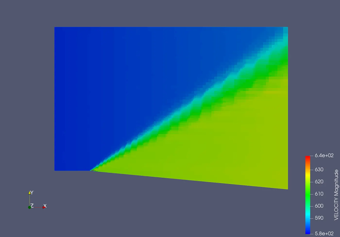
Velocity contour
Temperature contour
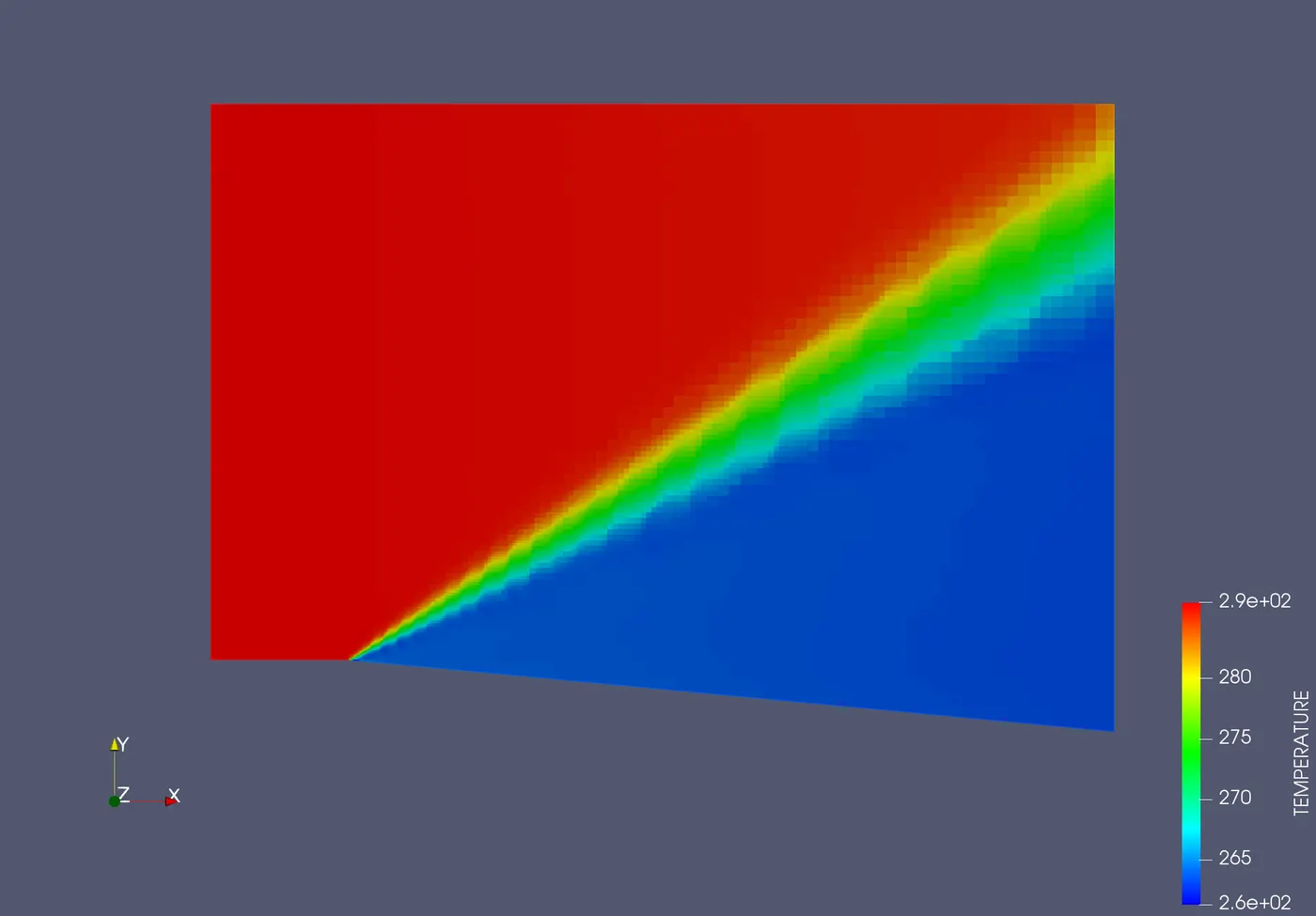
Temperature animation with adaptive mesh refinement
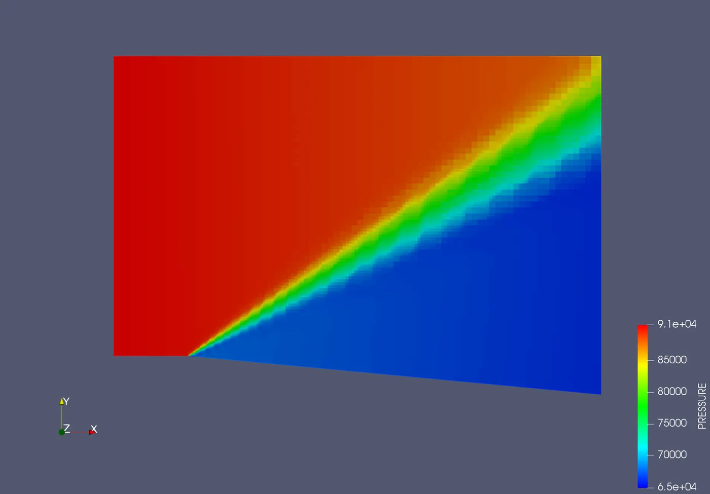
Pressure contour
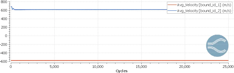
Velocity plot
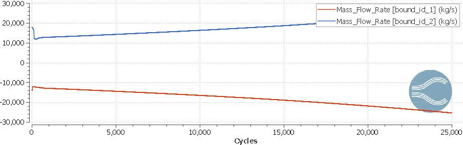
Mass flow rate
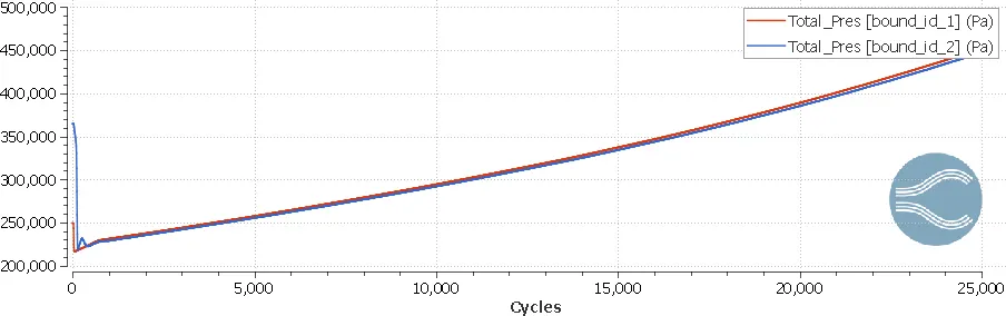
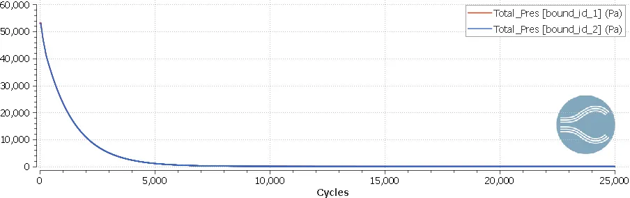
Total pressure plot
Case 2 (supersonic flow)
Grid control
Adaptive mesh refinement
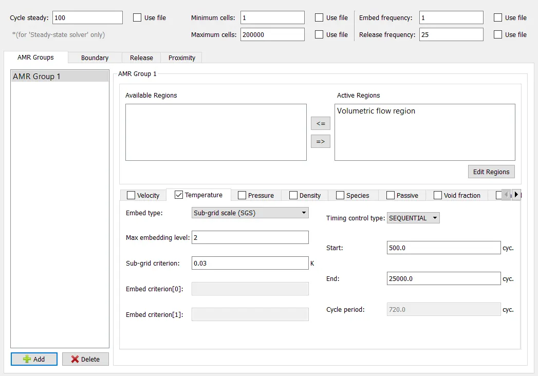
Mesh generated for SGS = 0.03 k
Results
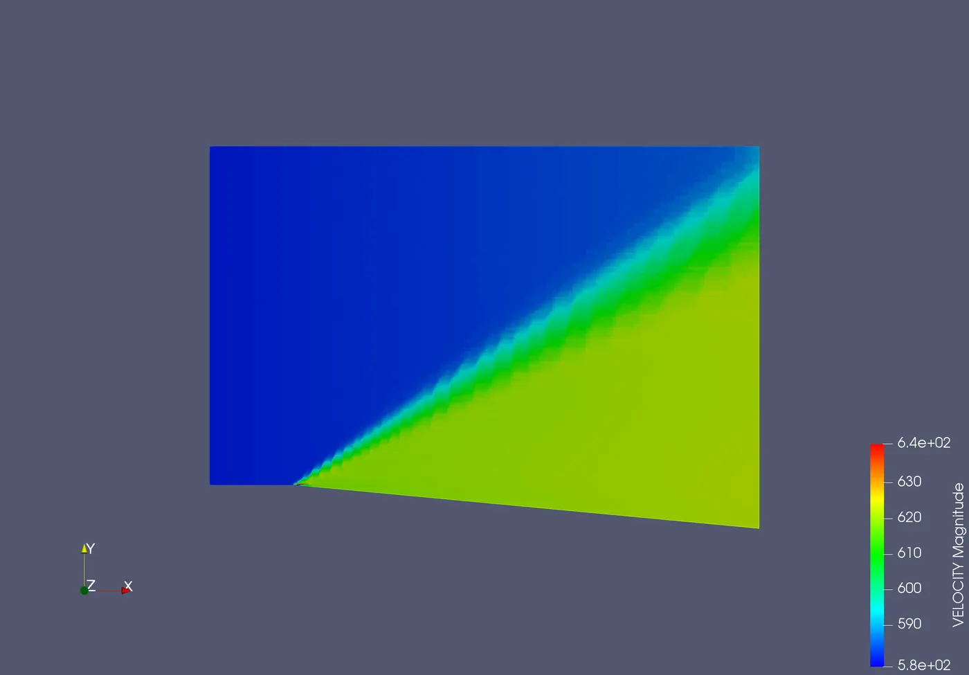
Velocity contour
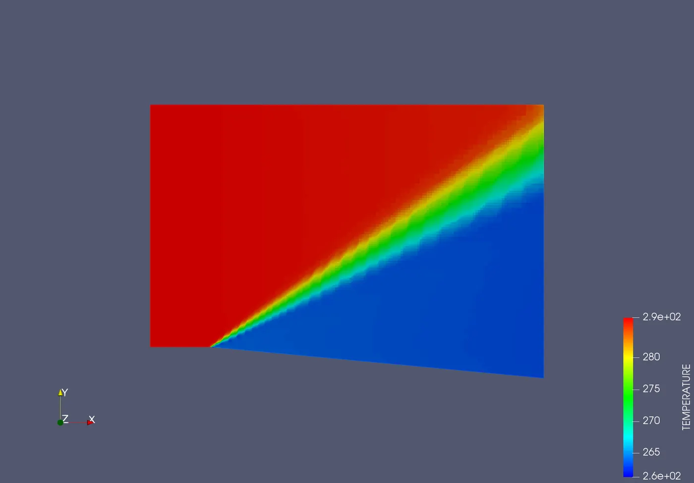
Temperature contour
Temperature animation with adaptive mesh refinement
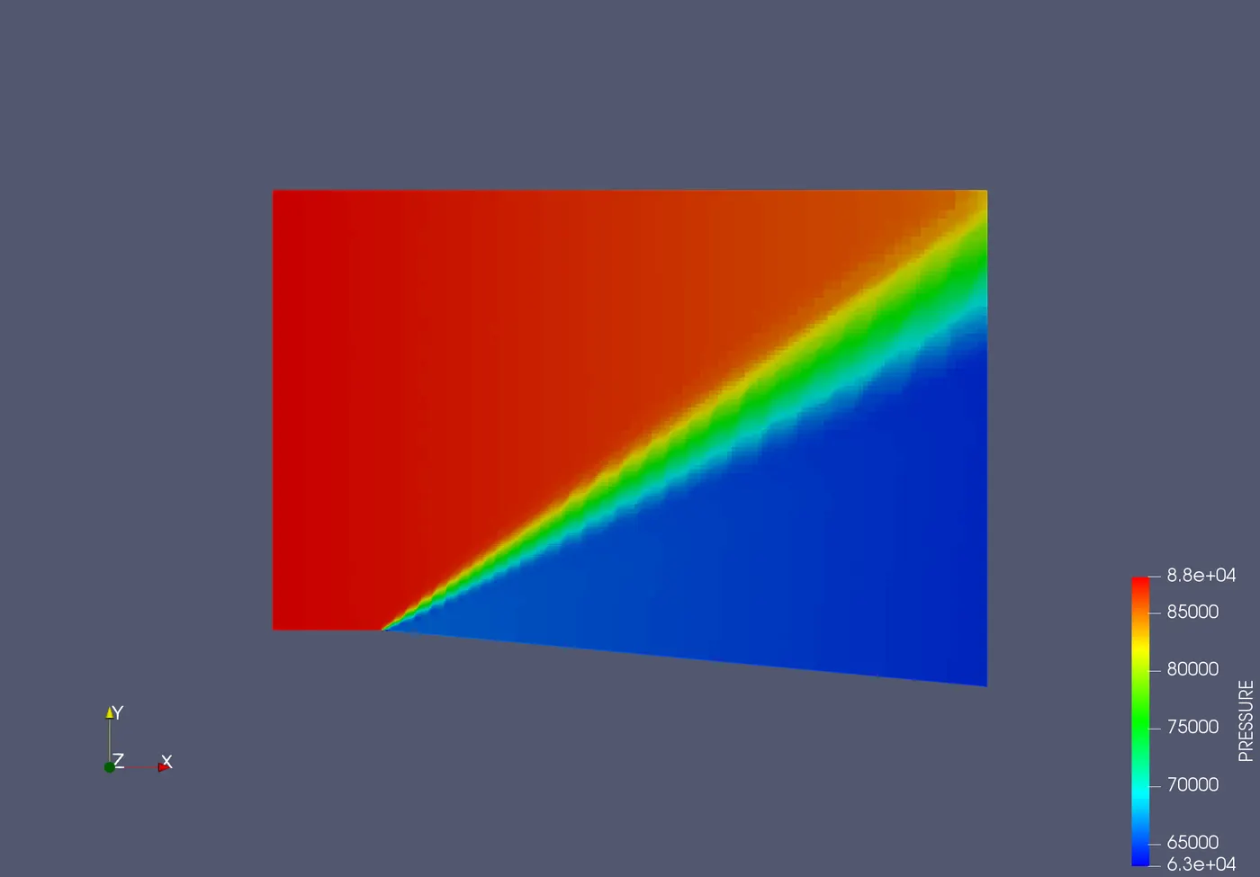
Pressure contour
Velocity plot
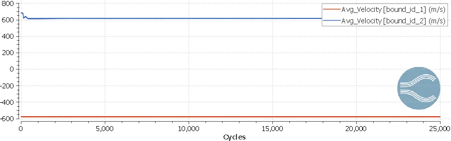
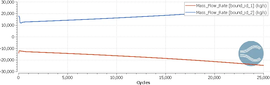
Mass flow rate plot
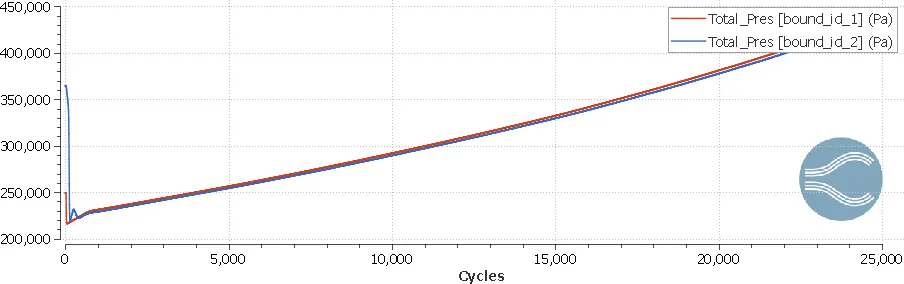
Total pressure plot
Case 3 (subsonic flow)
Grid control
Adaptive mesh refinement
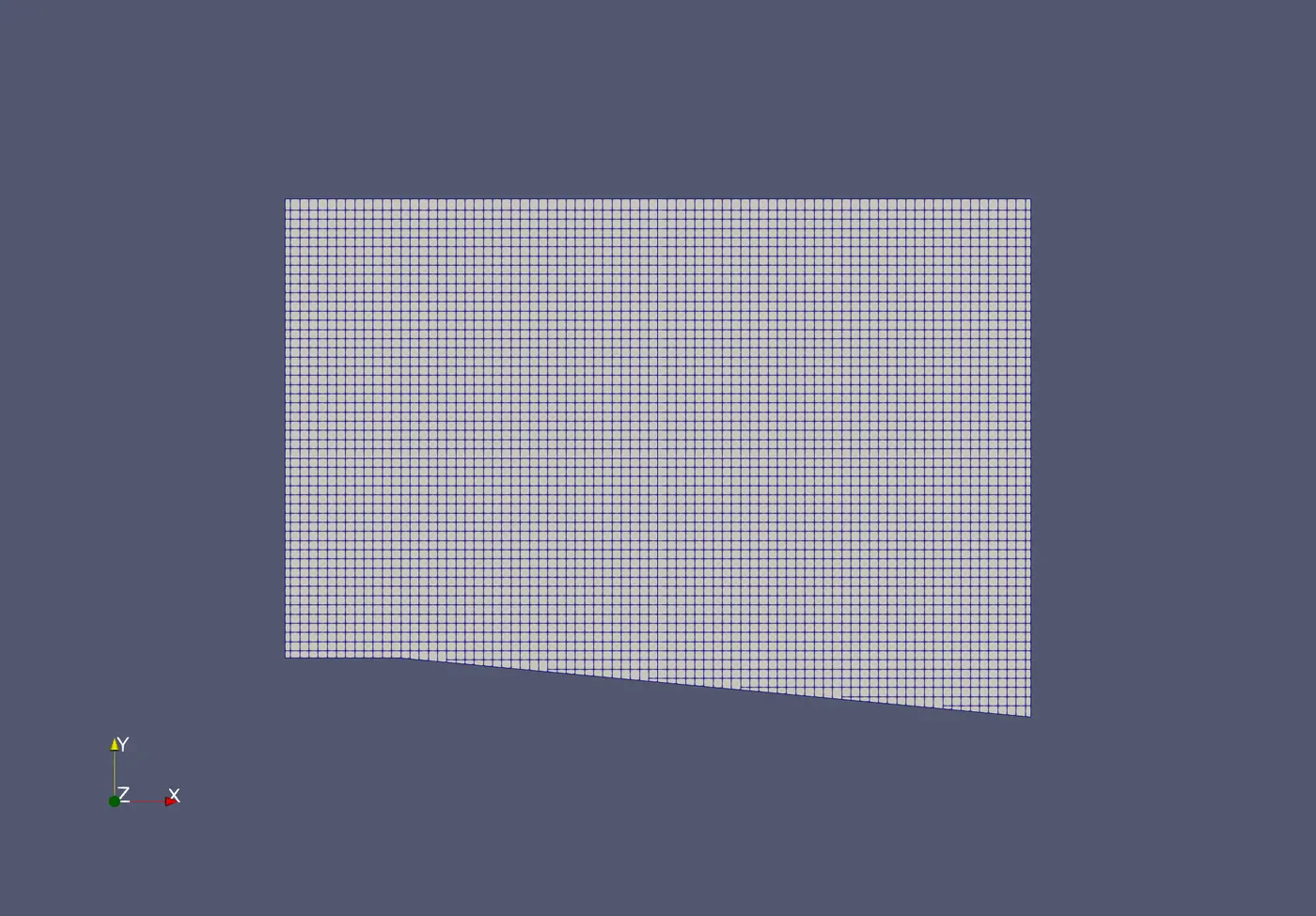
Mesh generated
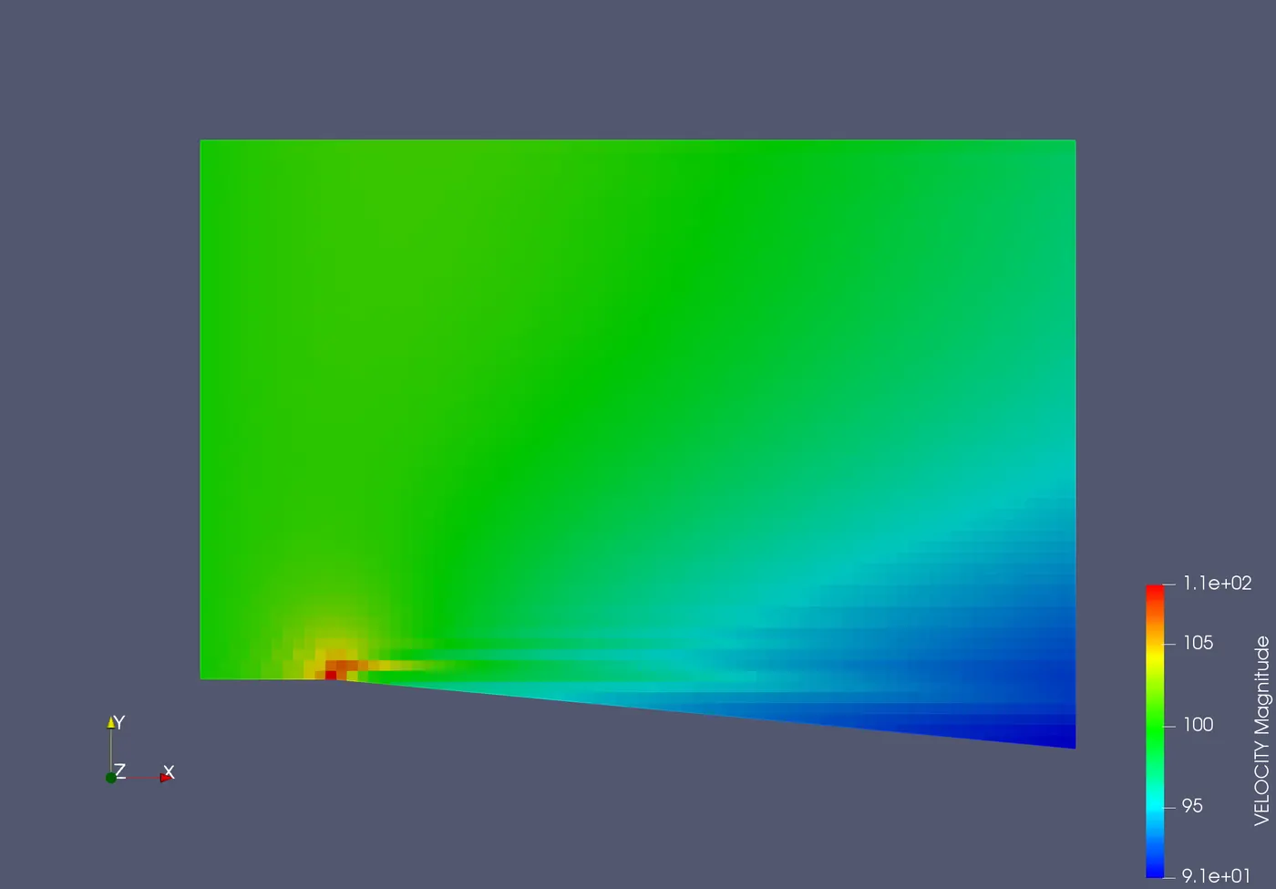
Velocity contour
Temperature contour
Pressure contour
Velocity plot
Mass flow rate plot
Total pressure plot
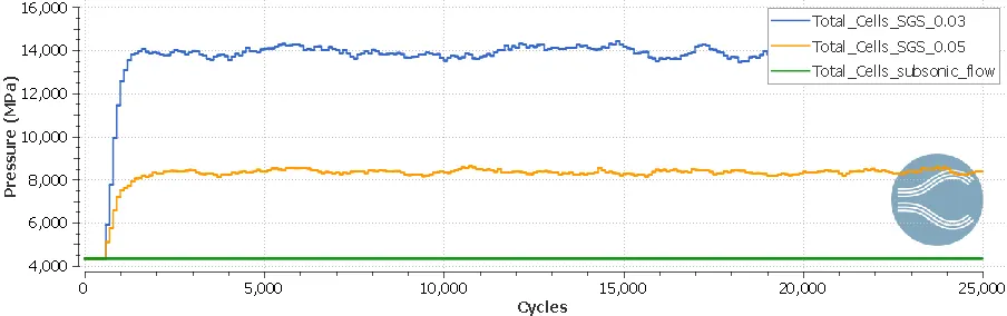
Comparing the total number of cells generated from case 1, case 2 and case 3
Conclusion:
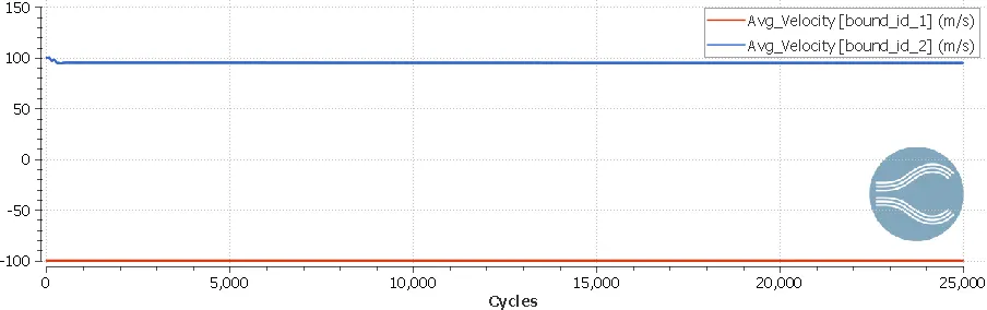
1. In subsonic flow, the fluid stream sense the change in shape of flow domain and adjust themselves ahead of it and flow around it smoothly. This is due to the fact that the fluid velocity is lower than the local speed of sound. In supersonic flow, the fluid stream feels the change in fluid domain shape when they reach the surface and hence, the fluid stream deviate. This phenomenon is observed clearly in the velocity contour and the vector plot shown below.
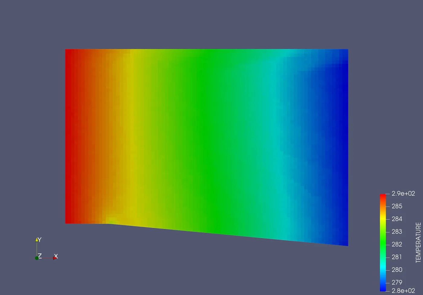
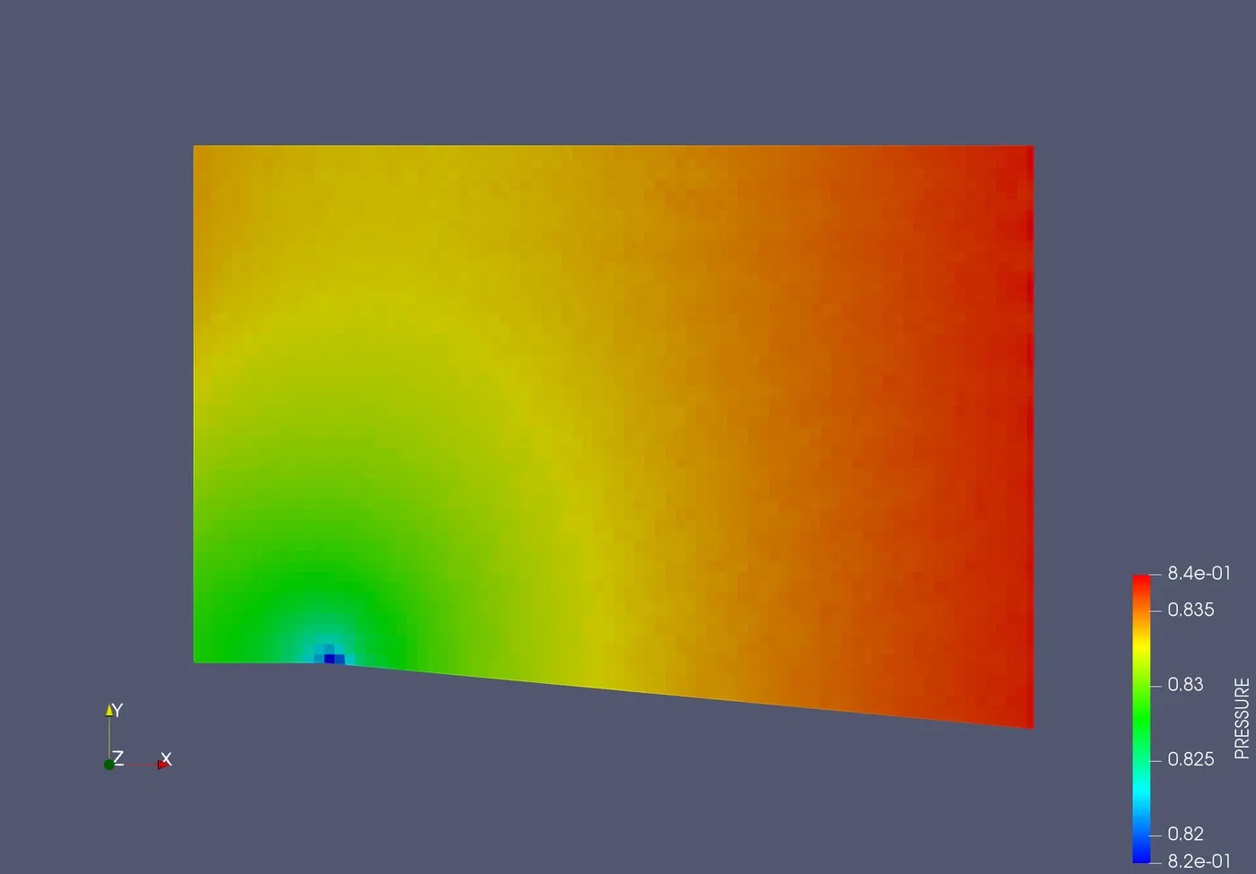
2. For subsonic flow, it can be seen from the pressure contour and temperature contour from case 3 that the pressure increases and temperature decreases as the fluid changes its direction gradually. For supersonic flow, the pressure and temperature both decrease as there is sudden change in flow direction.
3. In supersonic flow (case 1 and case 2), the mach number of fluid flow near the outlet is greater than the mach number of fluid flow near inlet. Thus, convex corner is a means to increase the mach number for supersonic flow.
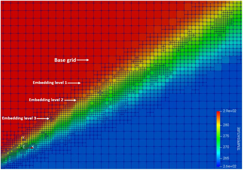
4. The above image shows the size of cells on base grid and embedding layers in the shock flow region. It can be seen that the size of cells decreases for higher embedding level.
5. It can be seen from the total cell count plot that the case 2 with sub-grid-scale equal to 0.03 generates more number of cells and refines mesh near the shock location. And no mesh refinement is done for subsonic flow, as there is no shock flow. Therefore, the lower sub-grid-scale value generates more number of cells and refines mesh.