Week 5: Prandtl Meyer Shock problem

Aim:

In the Prandtl Meyer shock problem, look at the effect of SGS temperature value on cell count and the shock location

Objectives:

1.Shock flow boundary conditions

Do a literature search on what BC's are typically used for shock flow problems

2. What is a shock wave?

In your own words, describe the physics behind shock waves

3. Effect of SGS parameter on shock location

QUES:1:

Shock Flow boundary conditions(BC):

1. Dirchlet
2. Neuman
3. Mixed
4. robin

Generally we use dirichelet and Neuman Boundary conditions for the most problems.

Dirchlet boundary conditions:

the Dirichlet (or first-type) boundary condition is a type of boundary condition, named after Peter Gustav Lejeune Dirichlet (1805–1859).[1] When imposed on an ordinary or a partial differential equation, it specifies the values that a solution needs to take along the boundary of the domain.

The question of finding solutions to such equations is known as the Dirichlet problem. In applied sciences, a Dirichlet boundary condition may also be referred to as a fixed boundary condition.

Applications

For example, the following would be considered Dirichlet boundary conditions:

In mechanical engineering and civil engineering (beam theory), where one end of a beam is held at a fixed position in space.

In thermodynamics, where a surface is held at a fixed temperature.

In electrostatics, where a node of a circuit is held at a fixed voltage.

In fluid dynamics, the no-slip condition for viscous fluids states that at a solid boundary, the fluid will have zero velocity relative to the boundary.

Neuman boundary conditions:

the Neumann (or second-type) boundary condition is a type of boundary condition, named after Carl Neumann.[1] When imposed on an ordinary or a partial differential equation, the condition specifies the values in which the derivative of a solution is applied within the boundary of the domain.

It is possible to describe the problem using other boundary conditions: a Dirichlet boundary condition specifies the values of the solution itself (as opposed to its derivative) on the boundary, whereas the Cauchy boundary condition, mixed boundary condition and Robin boundary condition are all different types of combinations of the Neumann and Dirichlet boundary conditions.

Applications

The following applications involve the use of Neumann boundary conditions:

In thermodynamics, a prescribed heat flux from a surface would serve as boundary condition. For example, a perfect insulator would have no flux while an electrical component may be dissipating at a known power.

In magnetostatics, the magnetic field intensity can be prescribed as a boundary condition in order to find the magnetic flux density distribution in a magnet array in space, for example in a permanent magnet motor. Since the problems in magnetostatics involve solving Laplace's Equation or Poisson's Equation for the magnetic scalar potential, the boundary condition is a Neumann condition.

QUES:2:

Shock Wave:

In physics, a shock wave (also spelled shockwave), or shock, is a type of propagating disturbance that moves faster than the local speed of sound in the medium. Like an ordinary wave, a shock wave carries energy and can propagate through a medium but is characterized by an abrupt, nearly discontinuous, change in pressure, temperature, and density of the medium.

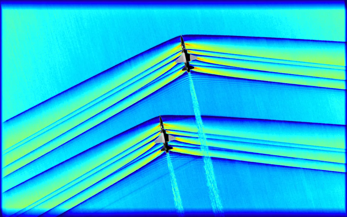
For the purpose of comparison, in supersonic flows, additional increased expansion may be achieved through an expansion fan, also known as a Prandtl–Meyer expansion fan. The accompanying expansion wave may approach and eventually collide and recombine with the shock wave, creating a process of destructive interference. The sonic boom associated with the passage of a supersonic aircraft is a type of sound wave produced by constructive interference.

Unlike solitons (another kind of nonlinear wave), the energy and speed of a shock wave alone dissipates relatively quickly with distance. When a shock wave passes through matter, energy is preserved but entropy increases. This change in the matter's properties manifests itself as a decrease in the energy which can be extracted as work, and as a drag force on supersonic objects; shock waves are strongly irreversible processes.

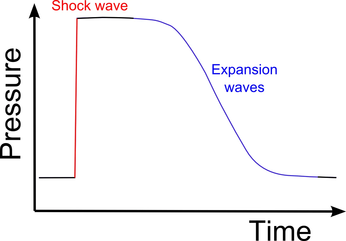
Advanced techniques are needed to capture shock waves and to detect shock waves in both numerical computations and experimental observations.

Computational fluid dynamics is commonly used to obtain the flow field with shock waves. Though shock waves are sharp discontinuities, in numerical solutions of fluid flow with discontinuities (shock wave, contact discontinuity or slip line), the shock wave can be smoothed out by low-order numerical method (due to numerical dissipation) or there are spurious oscillations near shock surface by high-order numerical method (due to Gibbs phenomena.

There exist some other discontinuities in fluid flow than the shock wave. The slip surface (3D) or slip line (2D) is a plane across which the tangent velocity is discontinuous, while pressure and normal velocity are continuous. Across the contact discontinuity, the pressure and velocity are continuous and the density is discontinuous. A strong expansion wave or shear layer may also contain high gradient regions which appear to be a discontinuity. Some common features of these flow structures and shock waves and the insufficient aspects of numerical and experimental tools lead to two important problems in practices:

(1) some shock waves can not be detected or their positions are detected wrong,

(2) some flow structures which are not shock waves are wrongly detected to be shock waves.

In fact, correct capturing and detection of shock waves are important since shock waves have the following influences:

(1) causing loss of total pressure, which may be a concern related to scramjet engine performance,

(2) providing lift for wave-rider configuration, as the oblique shock wave at lower surface of the vehicle can produce high pressure to generate lift,

(3) leading to wave drag of high-speed vehicle which is harmful to vehicle performance,

(4) inducing severe pressure load and heat flux, e.g. the Type IV shock–shock interference could yield a 17 times heating increase at vehicle surface,

(5) interacting with other structures, such as boundary layers, to produce new flow structures such as flow separation, transition, etc.

QUES:3:

Procedure:

Step:1

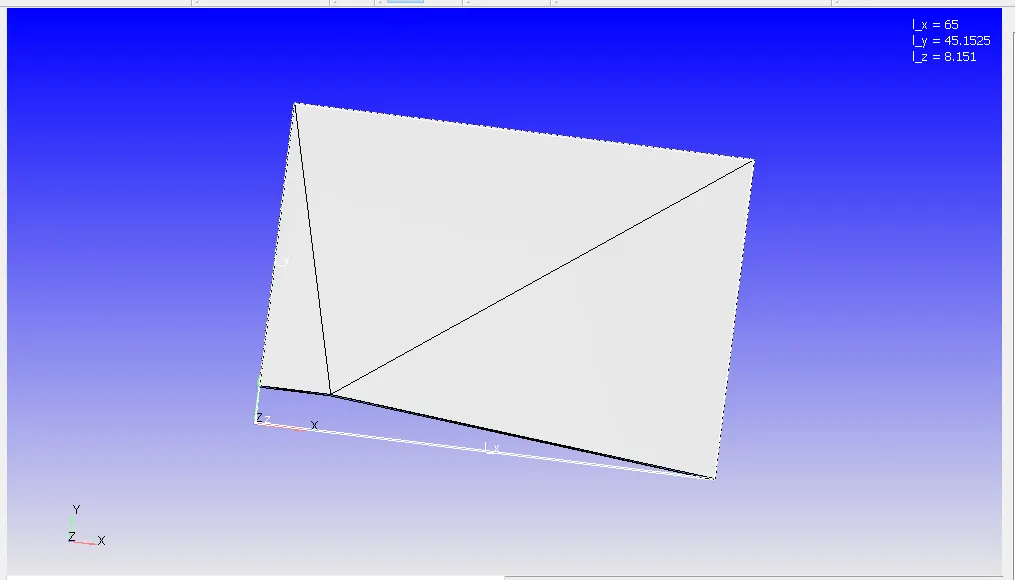
Import given geomentry And modify the geomentry suitable for smulation.

Step:2:

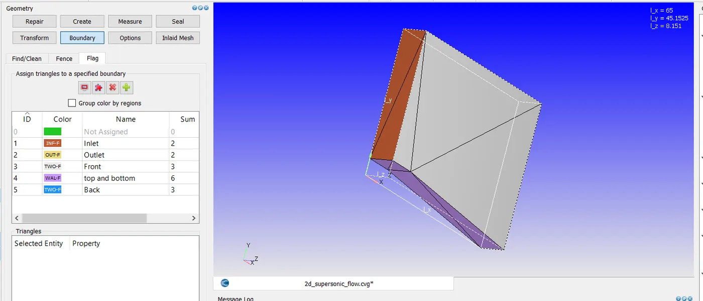
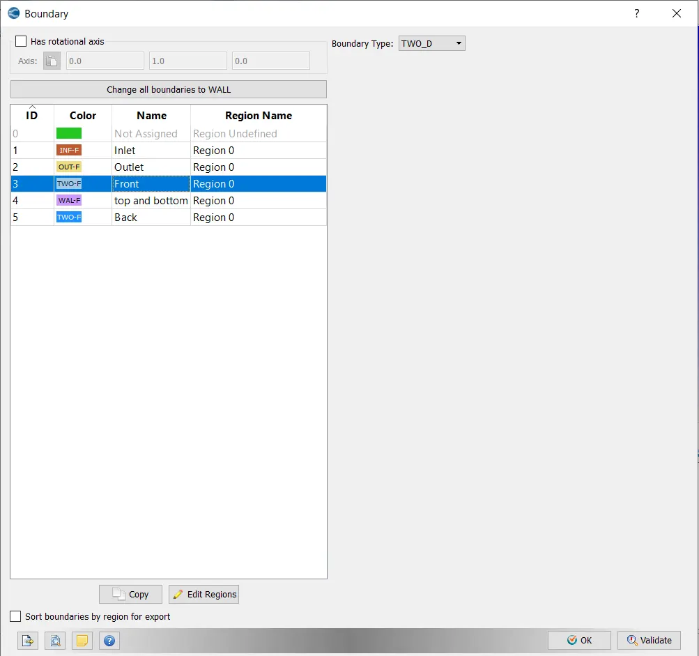
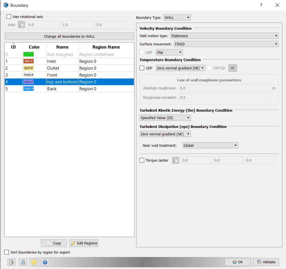
In this step, flag them together as boundaries which are marked with different colours.

Giving boundaries by selecting the sides which can help with other steps for simulation.

Once the boundaries have been flagged, we assign the different boundary conditions for the flow to take place within the geometry.

Step:3:

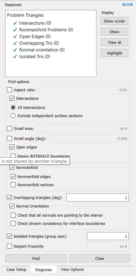
Check whether there is any errors by using diagnosis tool as shown below.

Step:4:

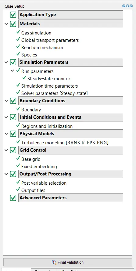
These are the following steps for setting up simulation .

Step:5:

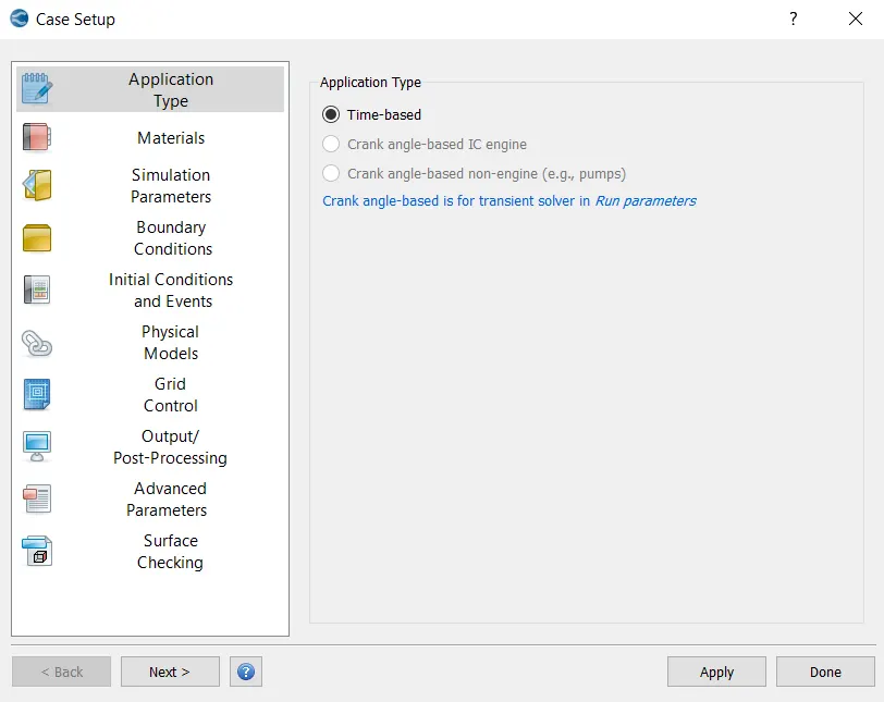
Select the application type time based for steady state simulation.

Step:6:

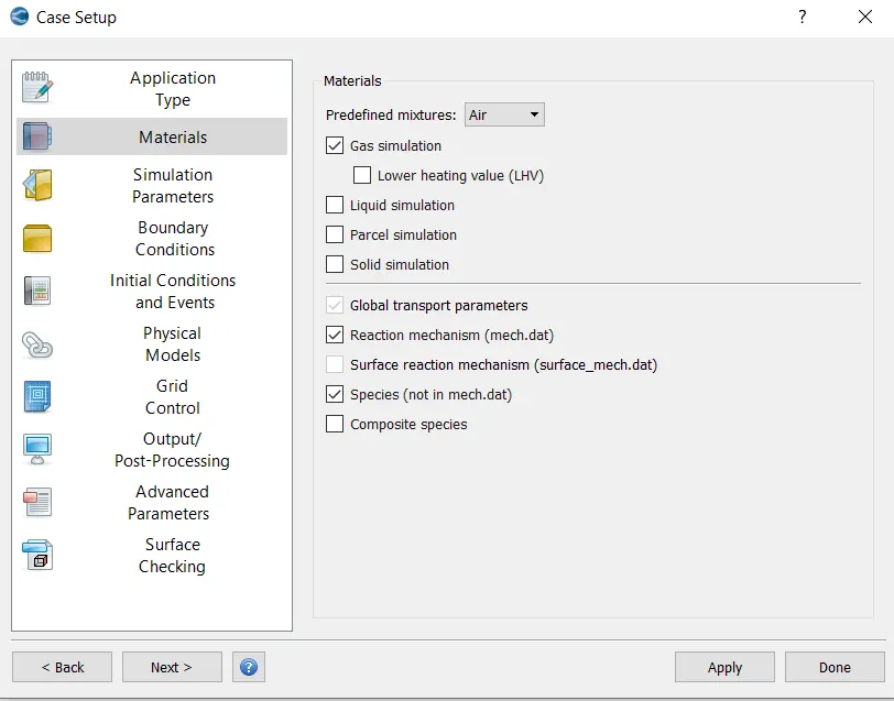
Select the material type for the flow through geomentry .here Air is the material taken.

Step:7

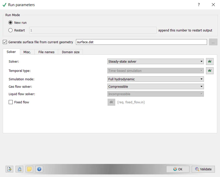
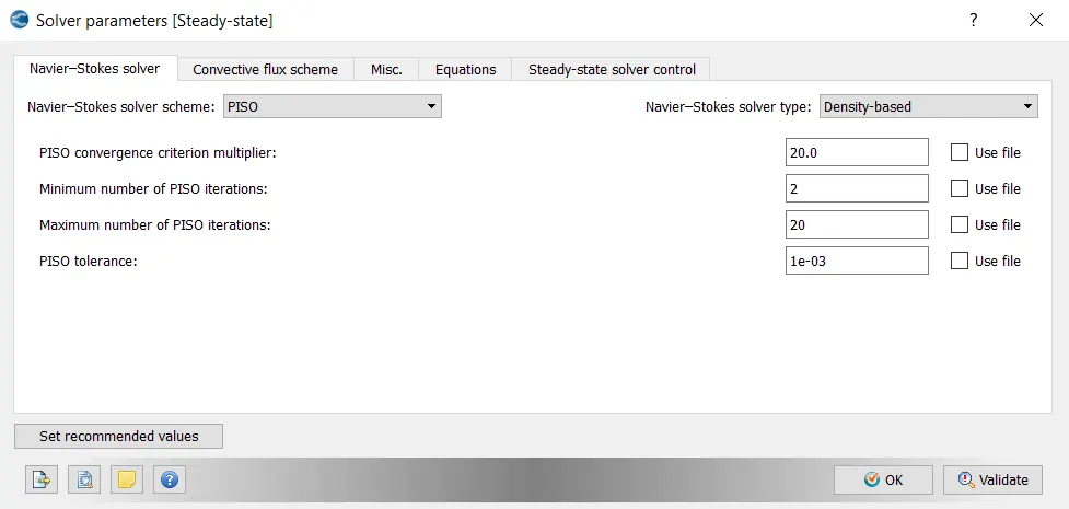
Select steady state solver for the simulation and density based solver parameters

Step:8

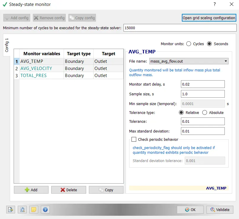
In Steady state monitor we can give minimum number of cycles for simulation .

Step:9:

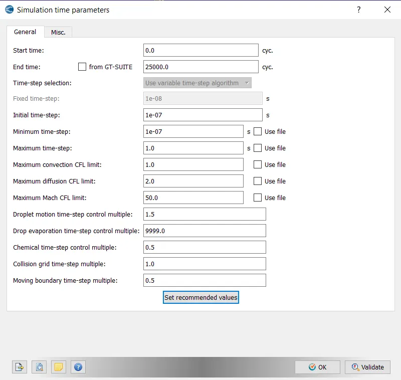
Here we can define the start and end time for cycles of simulation

and also the initial and minimum time step.

Step:10:

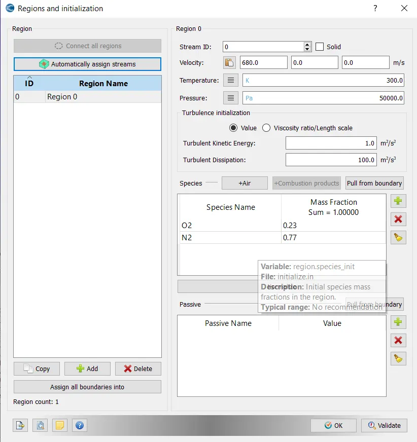
The boundaries are to bounded to a region for the steady simulation.so that volumetric region are created with the species of air.

here the simulation is supersonic so we have specify the velocity At the region.

Step:11:

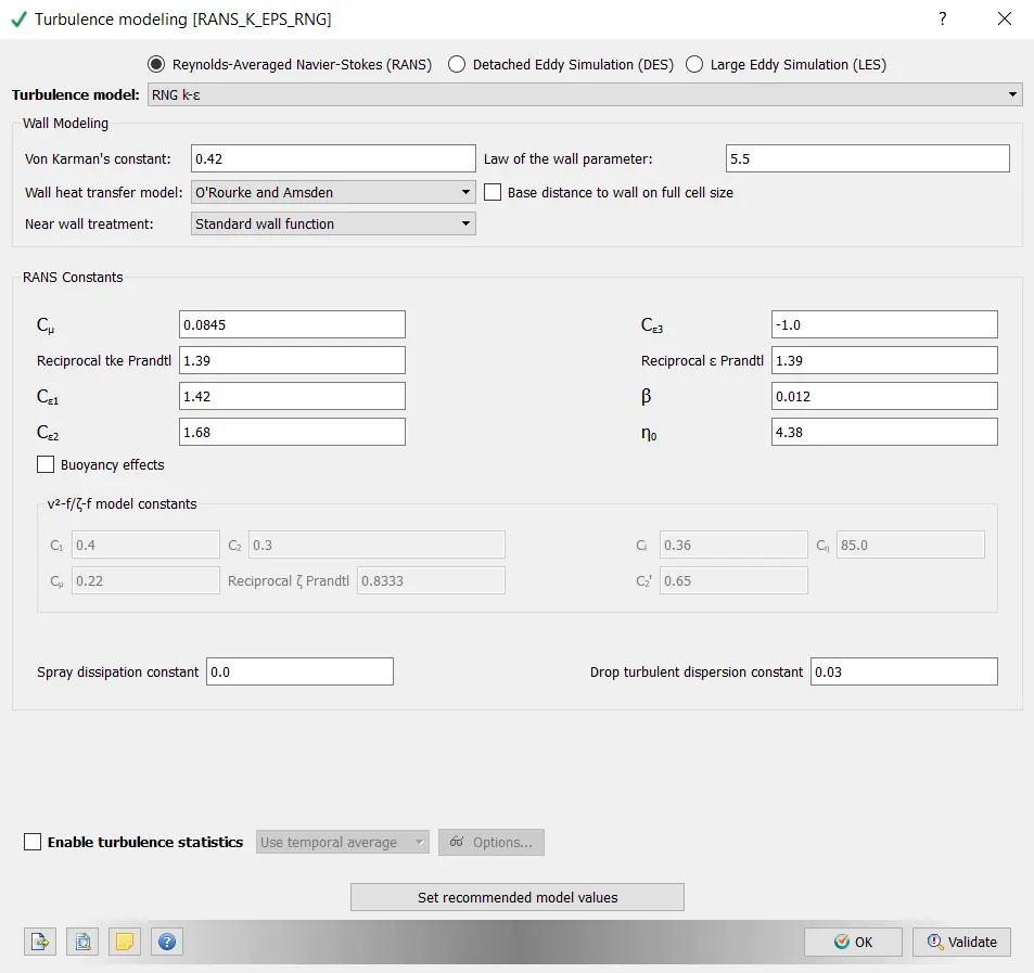
Here select the turbulance model that can be used for simulation.

Step:12:

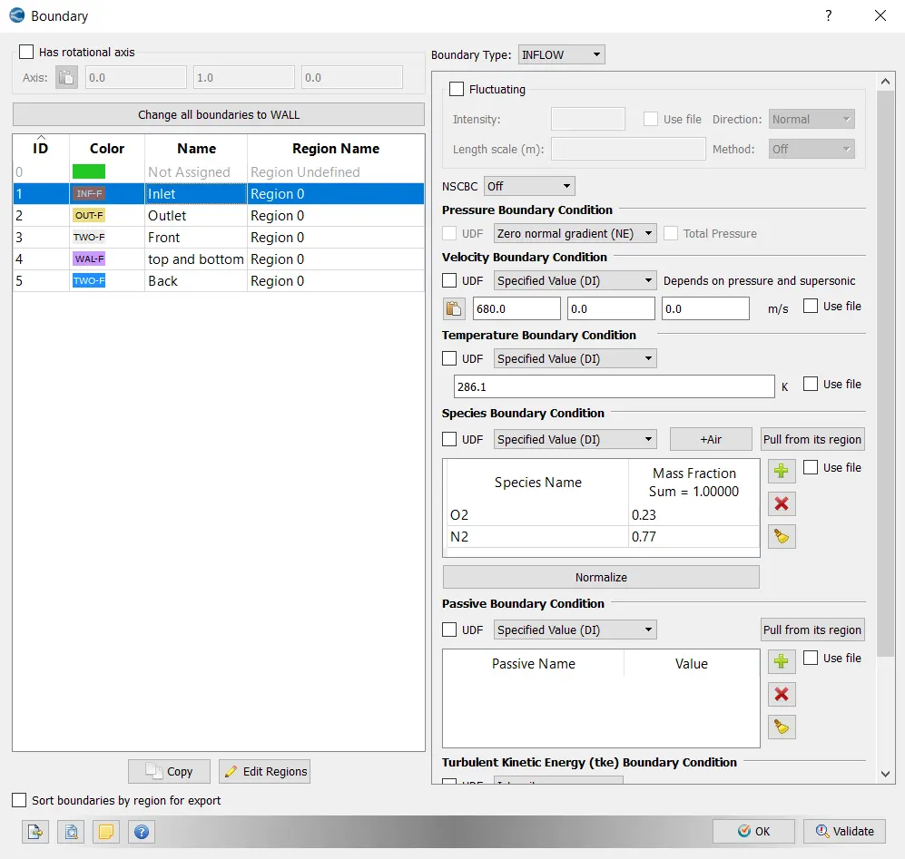
In here the boundary conditions are Assinged to the regions and also the inlet conditions are given .

pressure and temperature are defined for inlet.

Inlet:

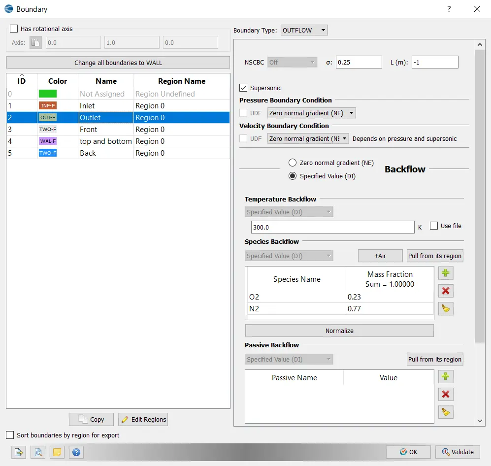
Outlet:

the Neumann (or second-type) boundary condition is a type of boundary condition, named after Carl Neumann.[1] When imposed on an ordinary or a partial differential equation, the condition specifies the values in which the derivative of a solution is applied within the boundary of the domain.

It is possible to describe the problem using other boundary conditions: a Dirichlet boundary condition specifies the values of the solution itself (as opposed to its derivative) on the boundary, whereas the Cauchy boundary condition, mixed boundary condition and Robin boundary condition are all different types of combinations of the Neumann and Dirichlet boundary conditions.

Front and back:

Top and bottom:

Step:13:

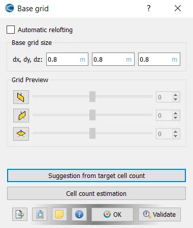
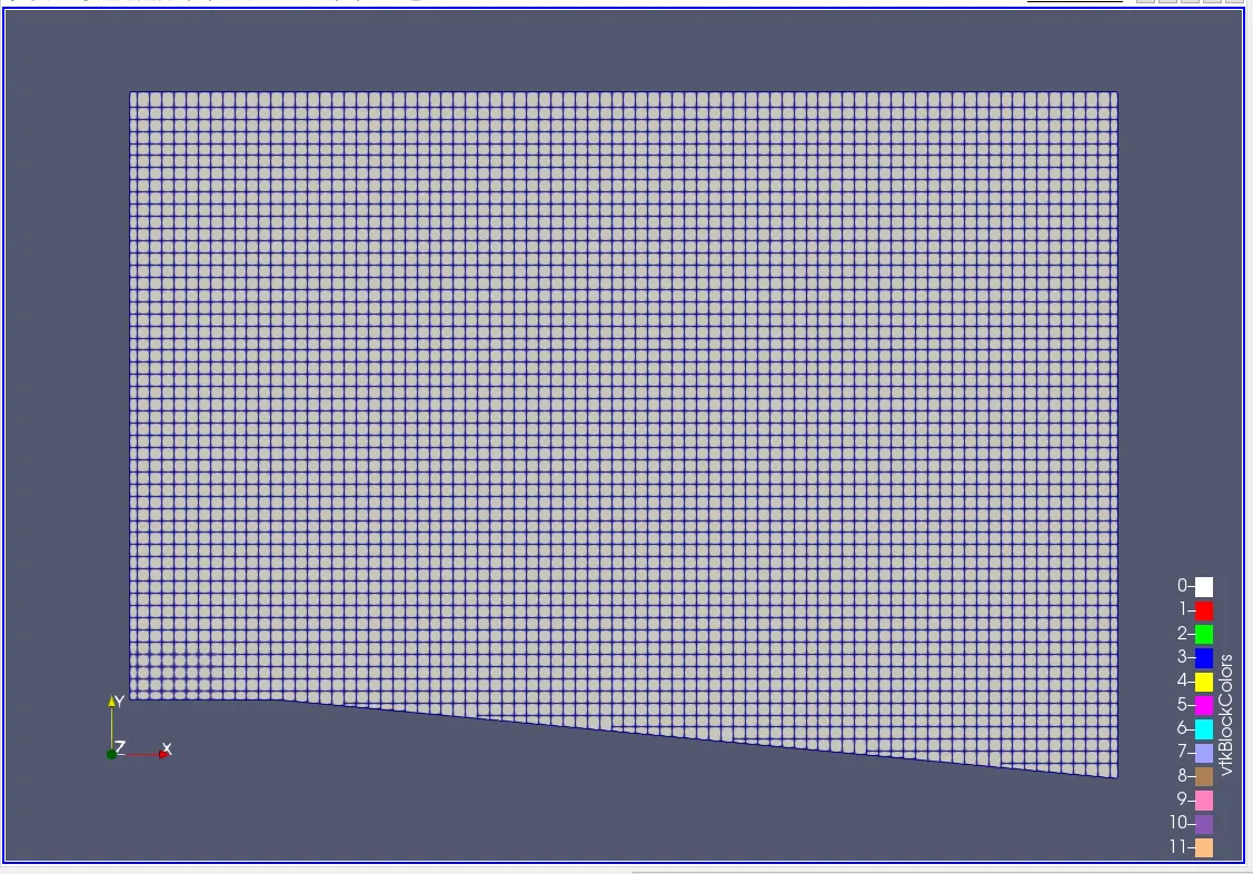
The basic mesh size of the Geomentry is specified here.

Step:14:

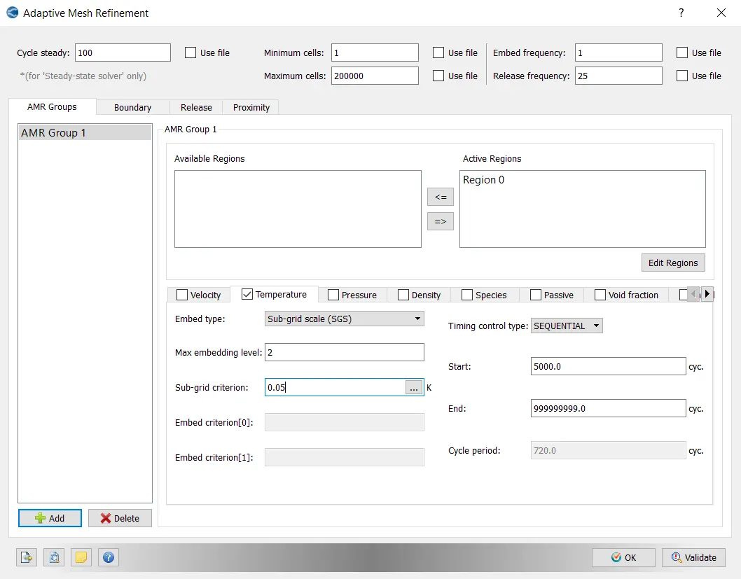
here In the AMR group teh active regions is selected and aslo the temperature AMR is set with maximum embedding level and sub grid criterion

Step:15:

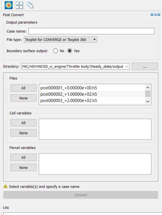
Post convert the files that is simulated in cygwin command window and file name is given .

Step:15:

Software used: ParaView As the simulation is binary files called “post” files are generated inside the output folder. These files have an extension *.out. Now these files are written by CONVERGE. These files contain information regarding the 3D flow field. We use a special software called ParaView that can read this flow information. However, before ParaView can do this, the files have to be converted to a form that ParaView can understand. This is done using a tool called post convert. After the conversion, we load the files into ParaView.

Results:

MESH:

Case :1:

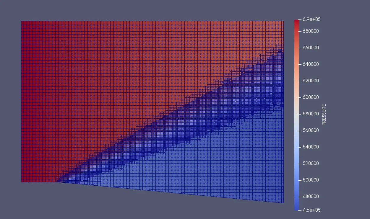
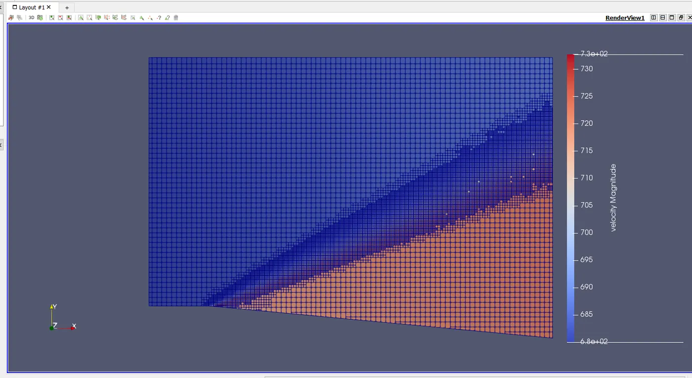
SGS = 0.01

Contours:

Pressure:

velocity :

Animation on SGS effect of Temperature contour:

Case :2:

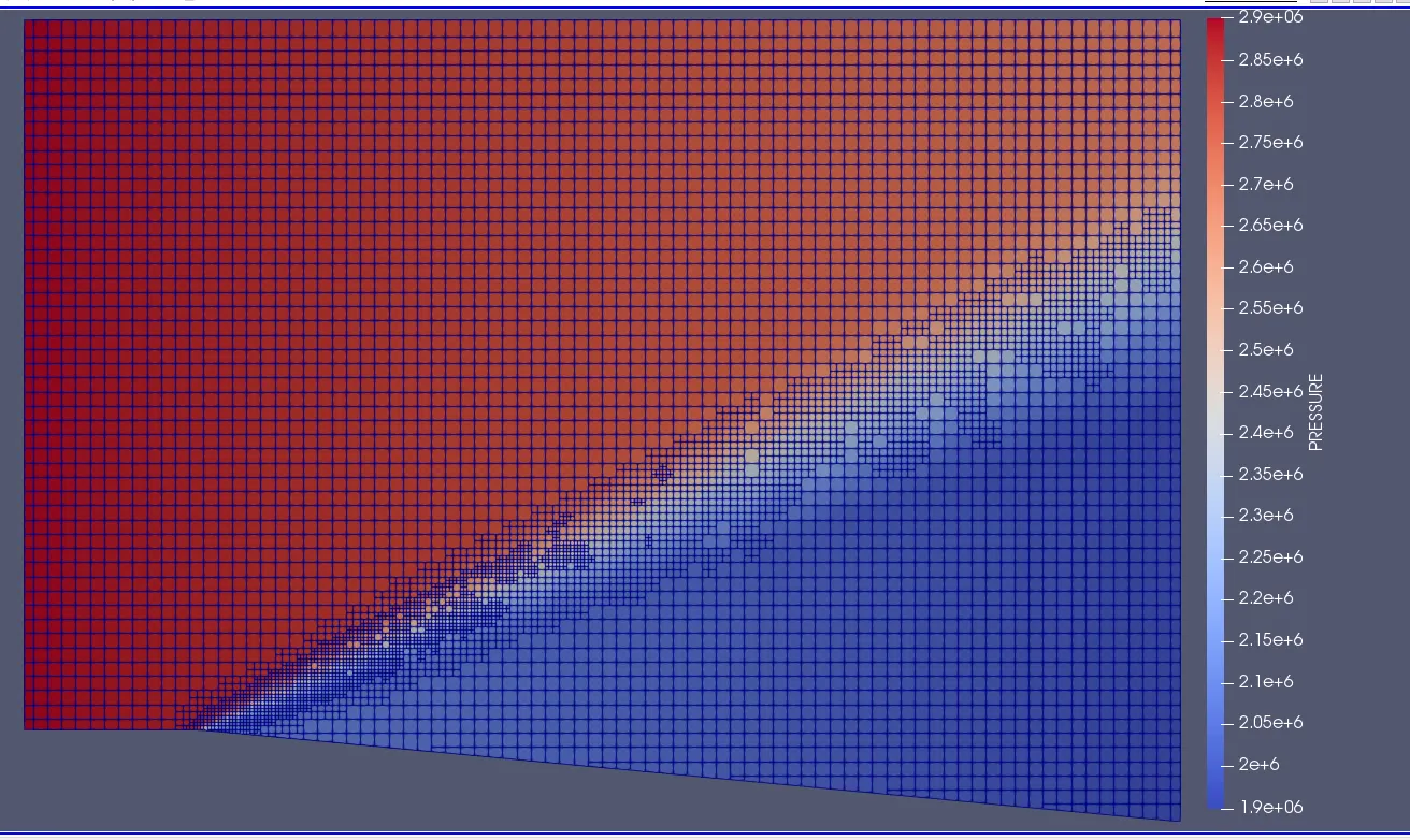
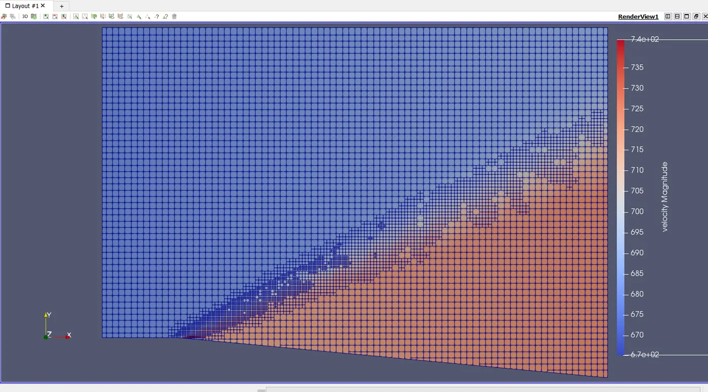
SGS = 0.05

Contours:

Pressure:

velocity :

Animation on SGS effect of Temperature contour:

Case :3:

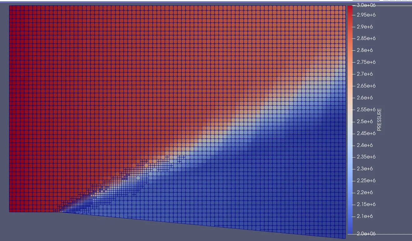
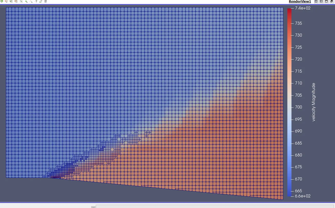
SGS = 0.1

Contours:

Pressure:

velocity :

Animation on SGS effect of Temperature contour:

CONCLUSION:

AS the SGS parameter decreases the total cell count increases.In other words for small SGS parameter, AMR refines the mesh for more number of cells in and Around the shock waves.

At shock location ,For high SGS parameter the mesh refinement area is very small and for small SGS parameter the mesh refinement area spans from sharp edge till the outlet boundary.

In supersonic Flow , the pandtl meyer expansion fan is clearly visible and the mesh refinement is also visible in shock region.