Week 5: Prandtl Meyer Shock problem

Aim: Prandtl Meyer Shock problem

Theory:

Neumann boundary condition:

The Neumann boundary condition specifies the normal derivative at a boundary to be zero or a constant. When the boundary is a plane normal to an axis, say the x axis, zero normal derivative represents an adiabatic boundary, in the case of a heat diffusion problem. Conduction heat flux is zero at the boundary. It may also represent a plane of symmetry.

The following applications involve the use of Neumann boundary conditions:

In thermodynamics, a prescribed heat flux from a surface would serve as boundary condition. For example, a perfect insulator would have no flux while an electrical component may be dissipating at a known power.

Dirichlet boundary condition:

The Dirichlet boundary conditions state the value that the solution function f to the differential equation must have on the boundary of the domain C. The boundary is usually denoted as ∂C.

In thermodynamics, where a surface is held at a fixed temperature.

In fluid dynamics, the no-slip condition for viscous fluids states that at a solid boundary, the fluid will have zero velocity relative to the boundary.

What is a shock wave?

In physics, a shock wave or shock, is a type of propagating disturbance that moves faster than the local speed of sound in the medium. Like an ordinary wave, a shock wave carries energy and can propagate through a medium but is characterized by an abrupt, nearly discontinuous, change in pressure, temperature, and density of the medium.

When a shock wave passes through matter, energy is preserved but entropy increases. This change in the matter's properties manifests itself as a decrease in the energy which can be extracted as work, and as a drag force on supersonic objects; shock waves are strongly irreversible processes.

Simulation setup Procedure:

Make sure the dimensions are as per the requirement when importing the geometry in converge.

Options > select geometry bounding box.

If not perform transformation.

In our case the entire geometry is transformed using a scaling factor of 0.001.

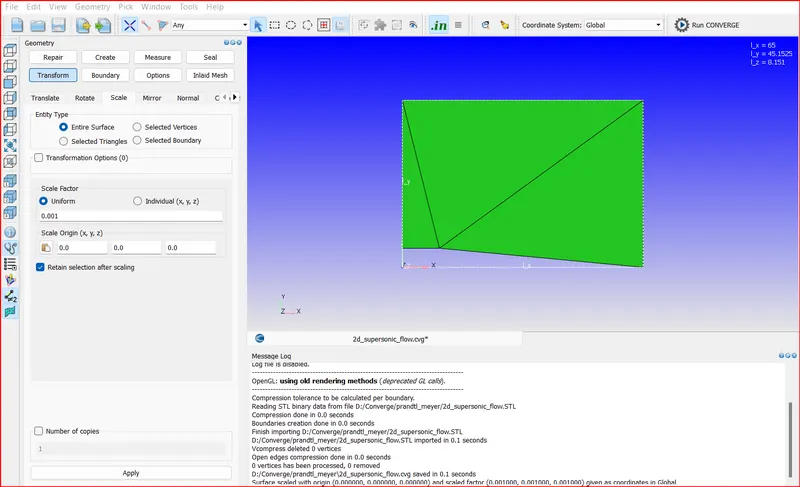
After running the diagnosis we can proceed with the case setup.

Case Setup:

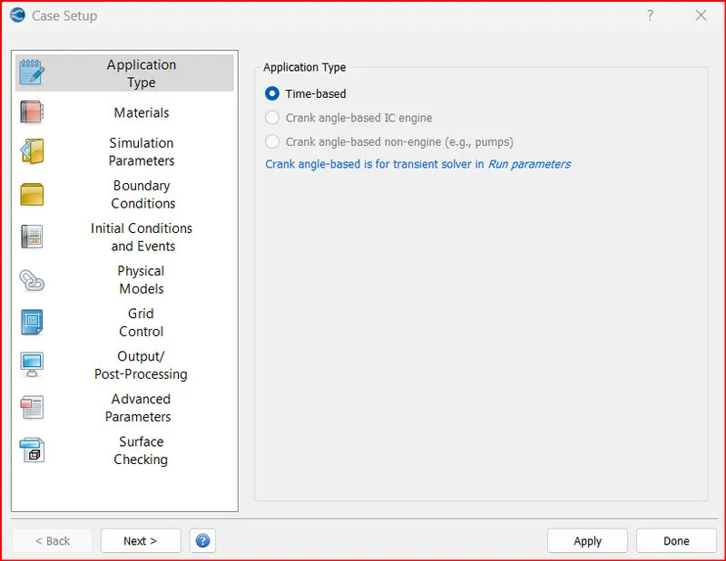
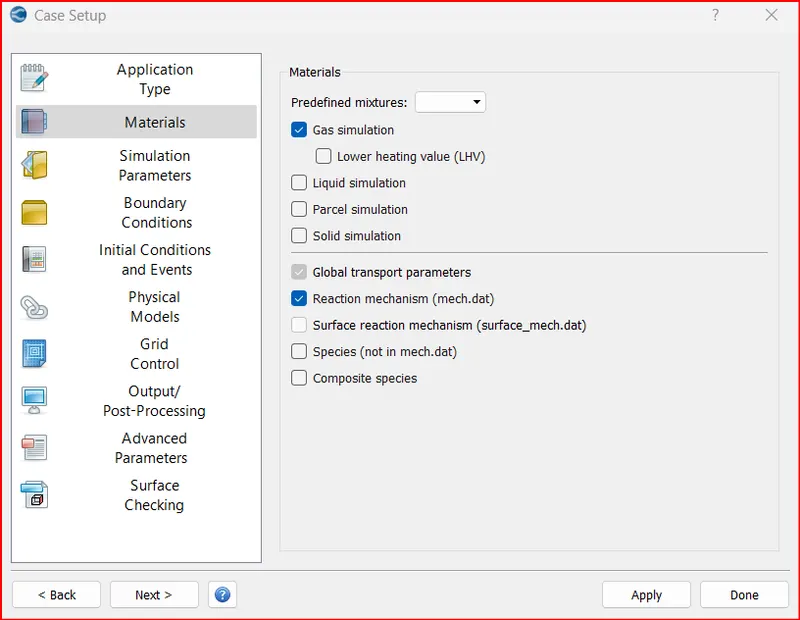
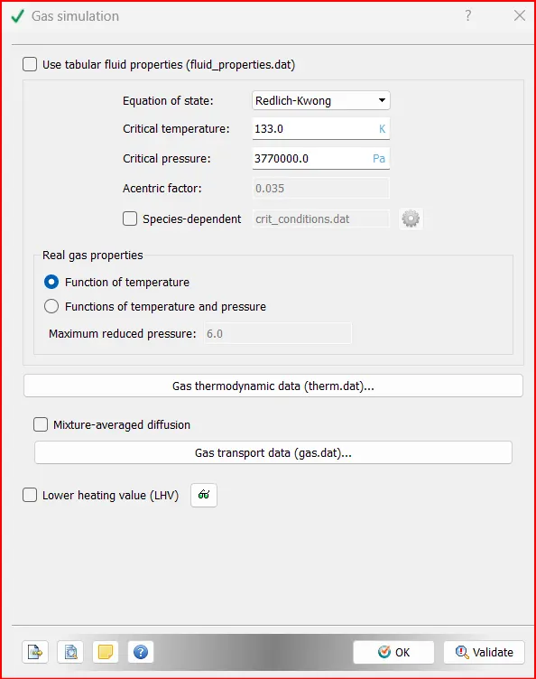
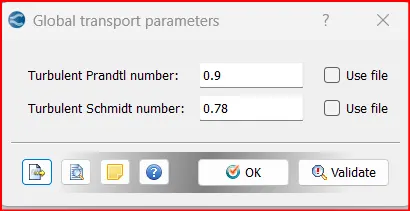
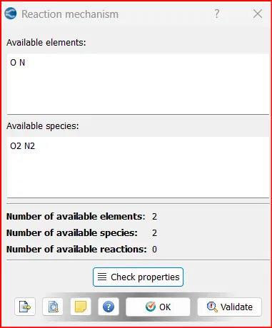
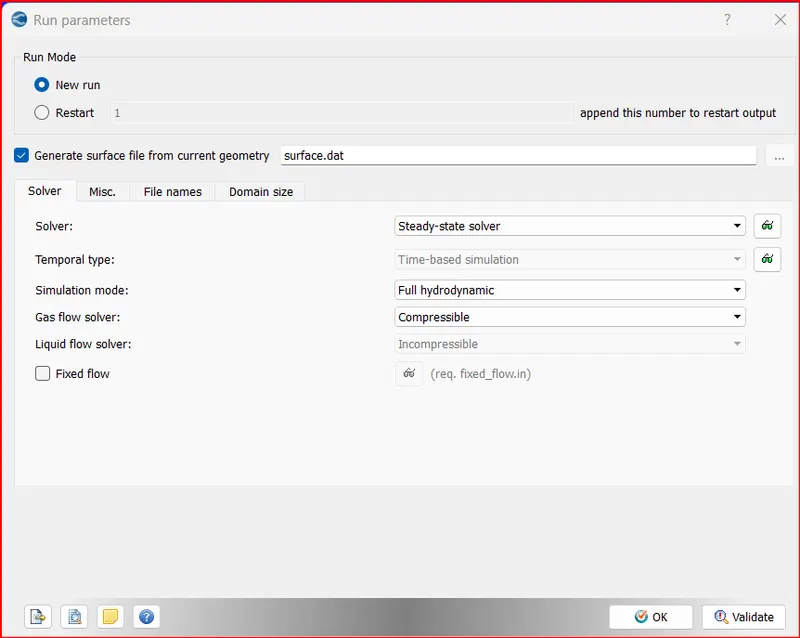
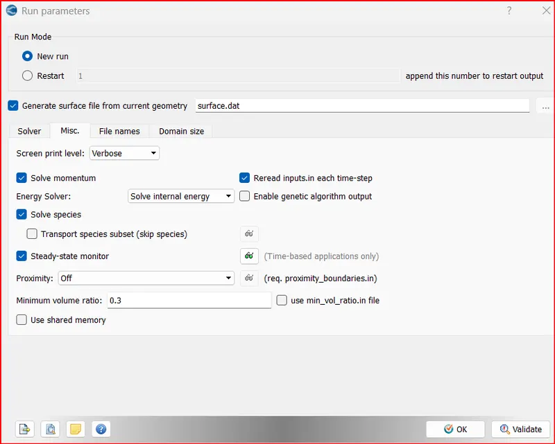
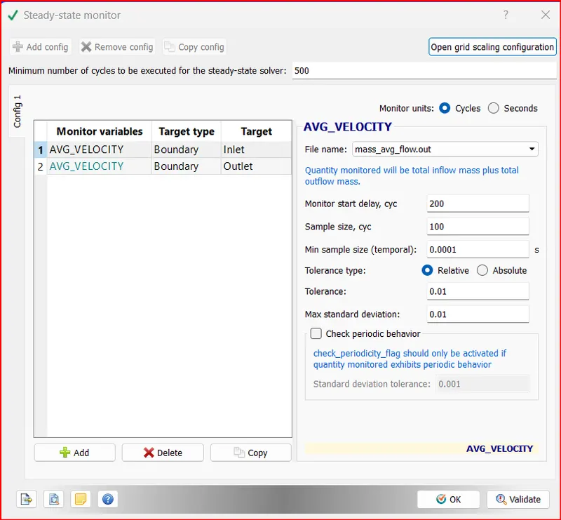
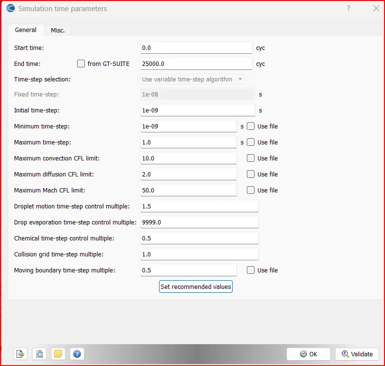
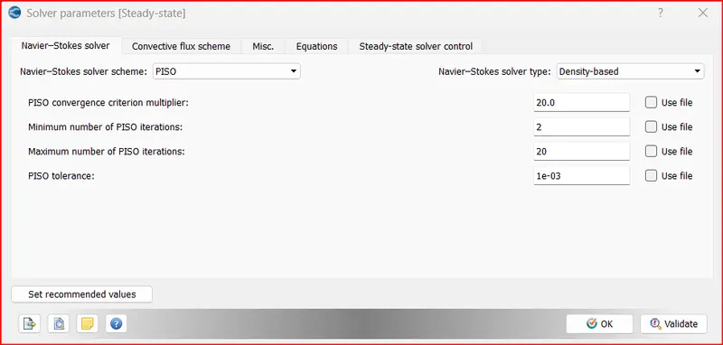
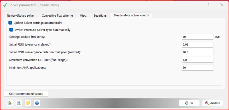
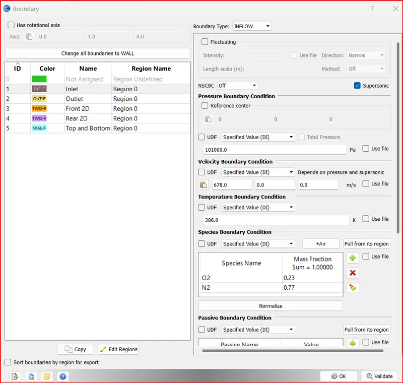
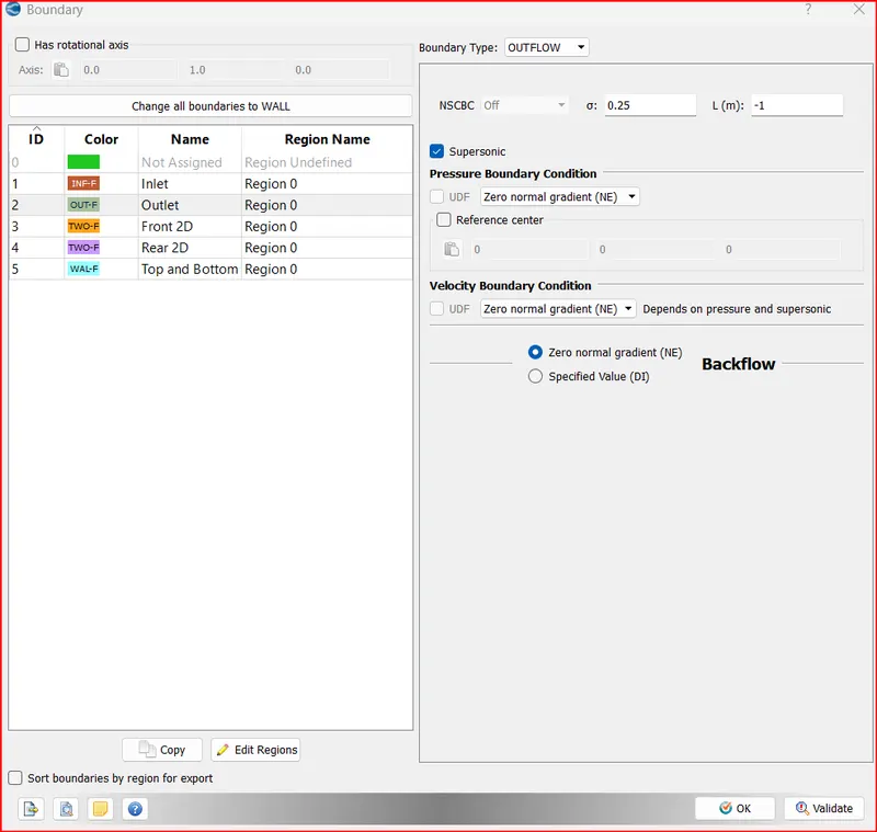
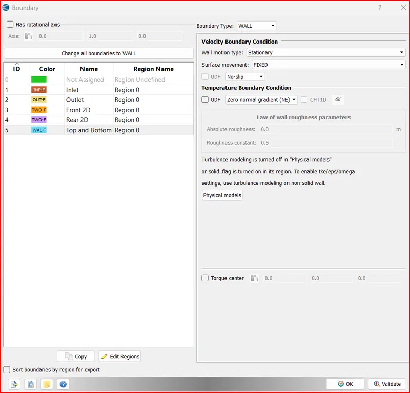
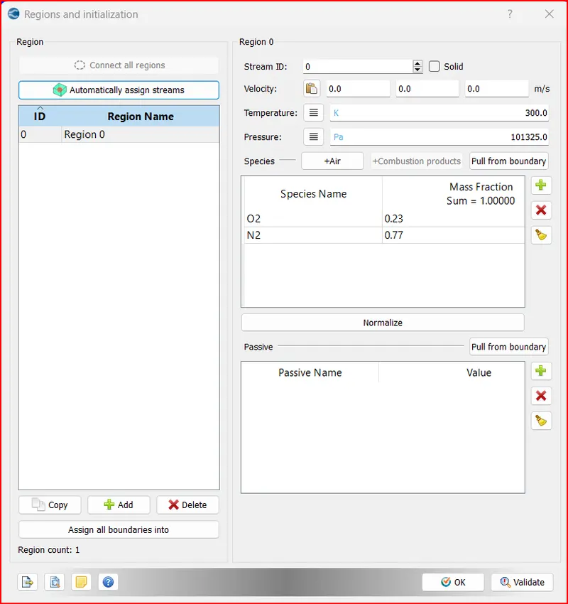
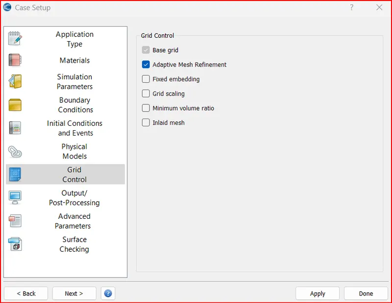
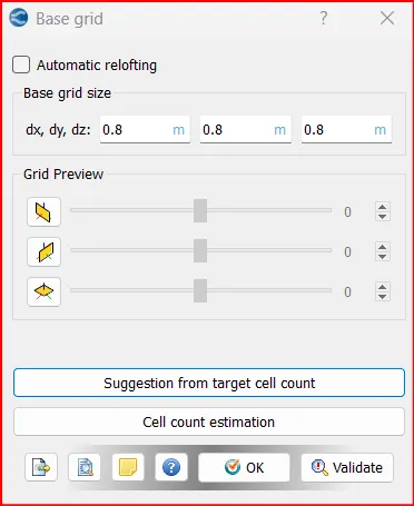
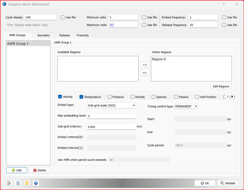
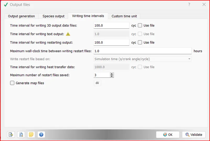
Post Processing:

Results:

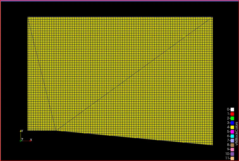
Mesh:

Velocity Animation:https://youtu.be/bjKv1tgM1yg