Week 5: Prandtl Meyer Shock problem
Aim:
To study the flow over the converge corner or expansion waves
To study the influence of SUB-GRID-CRITERION on the results
Literature review on boundary conditions and shock flow
To simulate the Prandtl -mayer Expansion wave
Prandtl-mayer Expansion Fan:
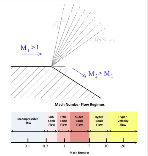
A supersonic expansion fan, technically known as prandtl-meyer expansion fan , a two dimensional simple wave, is a centered expansion process that occurs when a supersonic flow around a convex corner. The fan consists of an infinite waves , diverging from a sharp corner . when a flow turns around a smooth and circular corner , these waves can be extended backwards to meet at a point.
Each wave in the expansion fan turns the flow gradually ( in small steps) . It is physically impossible for the flow to turn through a single shock wave because this would violate the second law of thermodynamics.
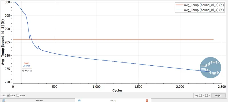
Across the expansion fan , the flow accelerates (velocity increases) and the mach number increases , while the static pressure, temperature and density decreases . since the process is isentropic the stagnation properties remain constant across the fan (I.e the total pressure and total temperature remains same)
Prandtl -Meyer expansion fans:
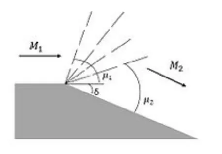
To this point , the only flow phenomena that have been discussed are shock waves, which slow the flow and increase its entropy . It is possible to accelerate supersonic flow in what has been termed a prandtl -Meyer expansion fan, after Ludwig Prandtl and Theodore Meyer
As opposed to the flow encountering an inclined obstruction and farming an oblique shock, the flow expands around a convex corner and forms an expansion fan through a series of isentropic mach waves. The expansion “fan “ is composed of mach waves that span from the initial Mach angle to the final Mach angle. Flow can expand around either a sharp or rounded corner equally , as the increase in Mach number is proportionally to only the convex angle of the passage. The expansion corner that produces the prandtl -Meyer fan can be sharp ( as shown in fig) or rounded . if the total turning angle is the same.
The prandtl-Meyer expansion can be seen as the physical explanation of the operation of the laval nozzle . The contour of the nozzle creates a smooth and continuous series of Prandtl -Meyer expansion waves.
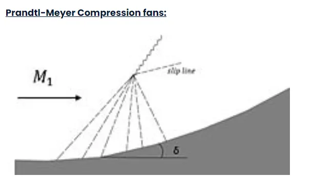
A prandtl Meyer compression is the opposite Phenomenon to a parallel prandtl - meyer expansion . if the flow is gradually turned through a angle of delta , a compression fan can be formed . This fan is a series of Mach waves that eventually coalesce into oblique shock. Because the flow is defined by an isentropic region( flow that travels through the fan ) and an isentropic region ( flow that travels through the oblique shock), a slip line results between the flow regions.
Boundary Conditions:
In CFD Boundary Conditions (BC) are equally important the governing equations , even if most text books deal predominantly with the governing equations only. From methametical point of view , boundary conditions are inherently linked with PDE’s . A PDE must have BC’s to obtain a unique solutions in CFD the various solutions to the same governing equations are distinguished by BC . In other words the flow over a car differs from the flow over a space shuttle exactly different BC are applied.
Specifying of wrong boundary conditions in the CFD imposing the solution to blown up or given a wrong Convergence solution.
Dirichlet Boundary Conditions:
In mathematics a Dirichlet problem is the problem of finding a function which solves a specified partial differential equation (PDE) in the interior of a given region that takes prescribed values on the boundary of the region.
The value of the dependent variable is specified on the boundary
Y=f
For example , if one end of an iron rod is held to absolute zero , then the value of the problem would be known at the point in space.
Neumann Boundary Conditions:
A boundary Conditions which specifies the value of the normal derivative of the function is a Neumann Boundary condition or second-type boundary condition.
dy/dx =f
For a example , if there is heater at one end of an iron rod , then energy would be added at a constant rate but the actual temp would not be known.
Robin Boundary Conditions:
Robin boundary conditions are a weighted combination of Dirichlet boundary and Neumann Boundary Conditions . this contrasts to mix boundary conditions , which are boundary conditions of different types specified on the different subsets of the boundary . Robin boundary conditions are also called impedance boundary conditions. From the applications in electromagnetic problems or convective boundary conditions from the application in heat transfer problems.
It is imposed on an ordinary or a partial differential equation, it is a specification of a linear combination of the values of a function and the valves of its derivative on the boundary of the domain.
Cauchy Boundary Conditions:
The Cauchy Boundary Conditions augments an ordinary differential equation or a partial differential equation with conditions that the solutions must satisfy on the boundary , ideally so to ensure that the unique solution exists .A Cauchy boundary condition specifies both the function values and normal derivative on the boundary of the domain. This corresponds to imposing both a Dirichlet Boundary Conditions and a Neumann Boundary conditions.
Cauchy boundary conditions are simple and commonly used in second -order ordinary differential equations.
Shock Wave:
When the speed of the moving object or source in a medium is exceeds the speed of the sound, then the wave fronts lag behind the object forming a cone shaped region with the source at the vertex behind the object. The edge of the cone forms supersonic wave front with a large amplitude which is called shock wave.
The shock wave carries the energy , Across a shock wave , the mach number decreases , the pressure increases and there is a loss in total pressure because the process is irreversible.Through a expansion fan , The Mach number increases , the static pressure decreases and the total pressure remains constant . Expansion fans are isentropic.
Shock waves are not conventional sound waves , A shock wave takes the form of a very sharp change in the gas properties , shock wave in air are heard as a loud “crack” or “snap” noise.
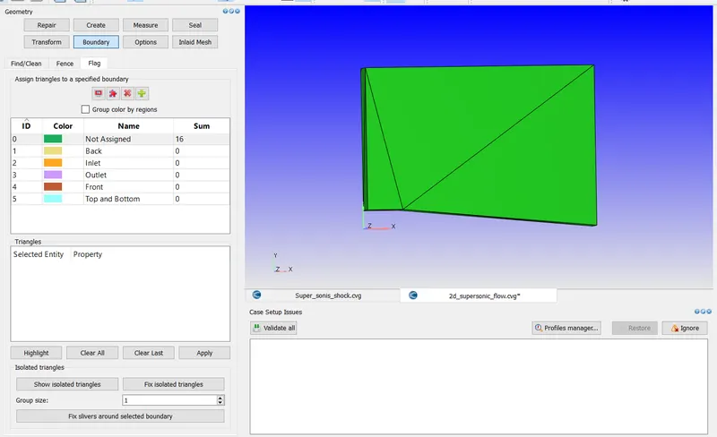
Importing The Geometry:
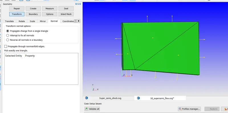
Vectors and Normal Setup:
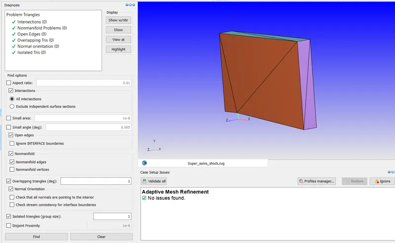
Diagnosis the Geometry:
Boundaries alignment: 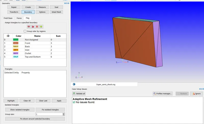
Case setup:
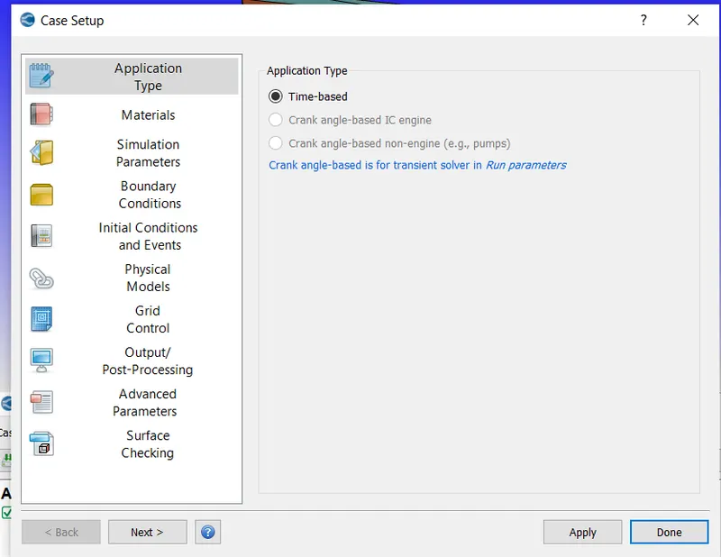
Material Selection:
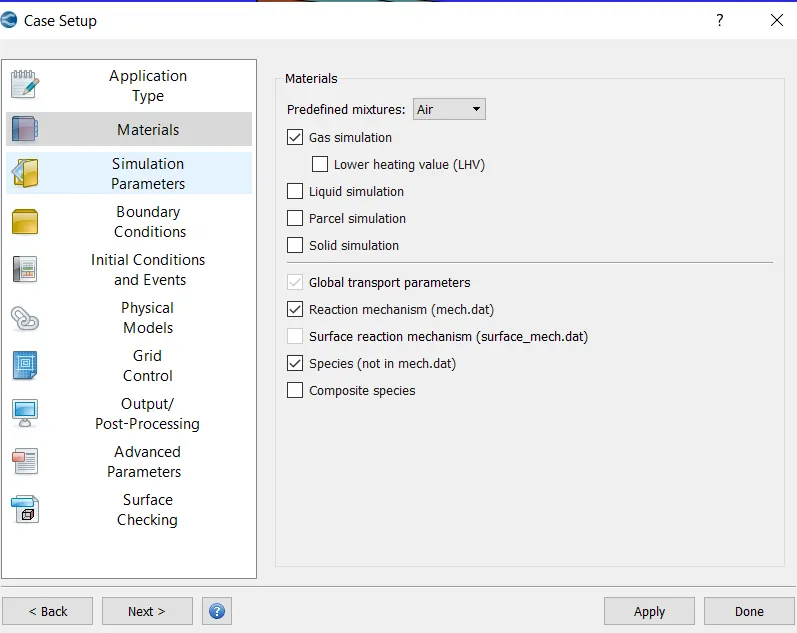
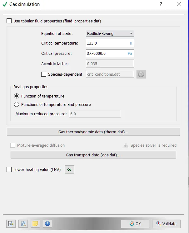
Gas simulation:
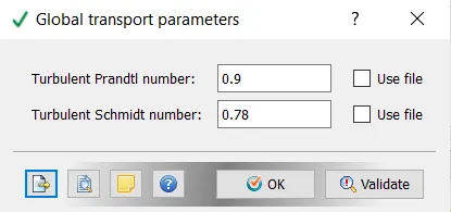
Global Transport properties:
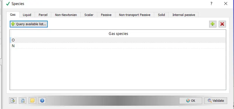
Species:
Simulation Parameters:
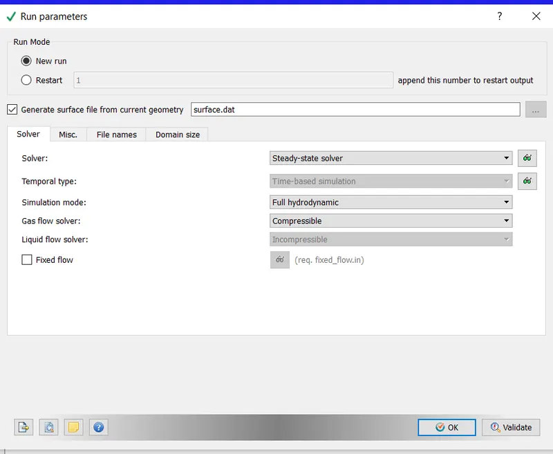
Run parameters:
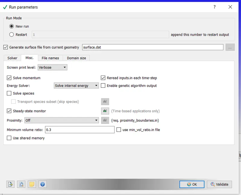
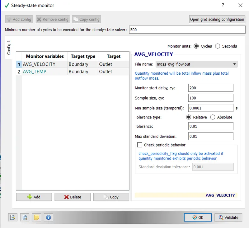
Steady State Monitor:
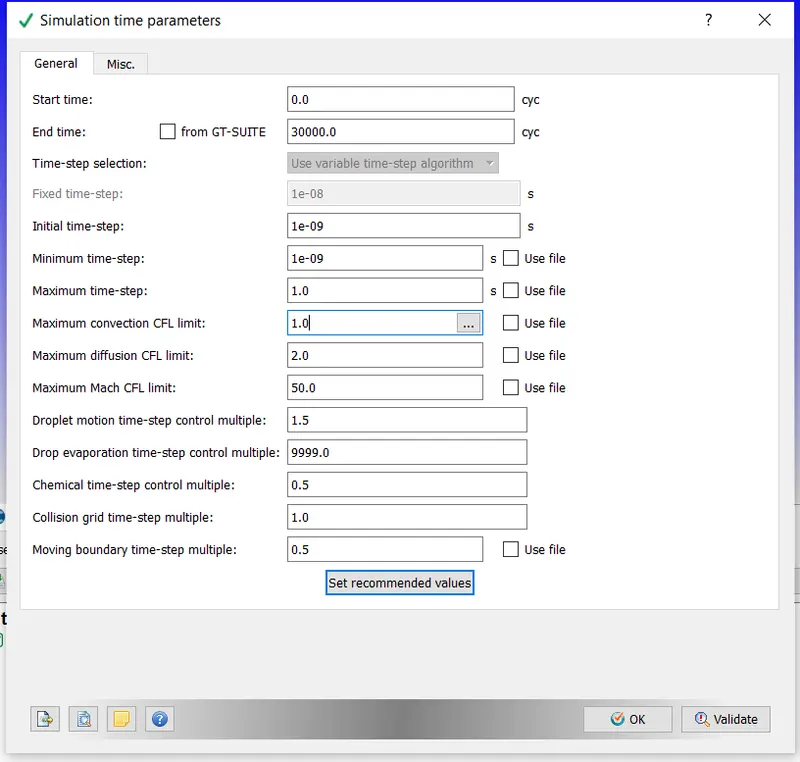
Simulation Time Parameters:
Solver Parameters:
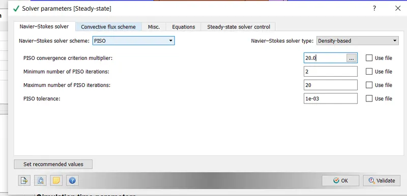
Initial and Boundary Conditions:
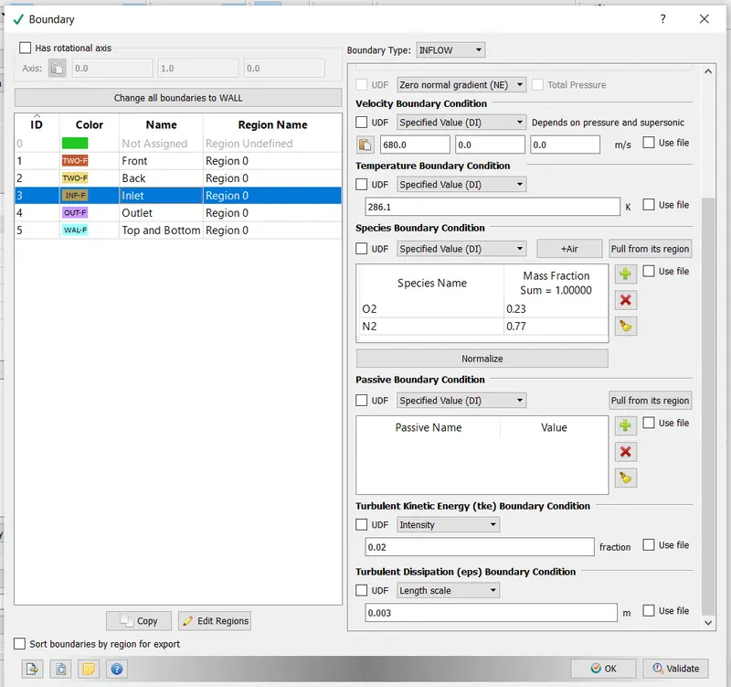
Inlet Boundary Conditions:
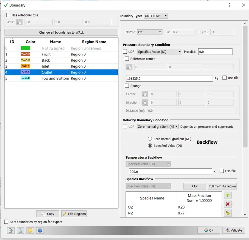
Outlet Boundary Conditions:
Front and Back
Two-D Boundary Conditions
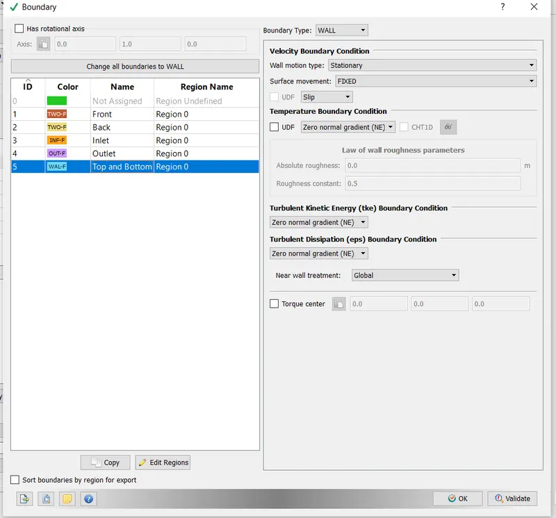
Top and Bottom Boundary Conditions:
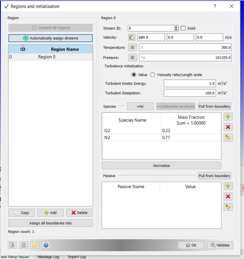
Regions and Initialization:
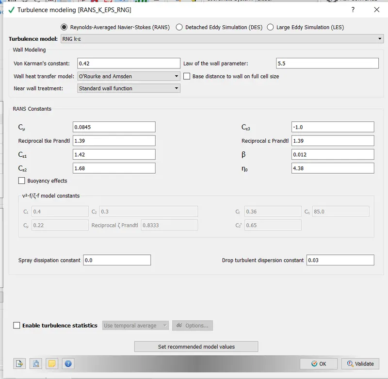
Physical models:
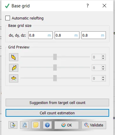
Grid Control:
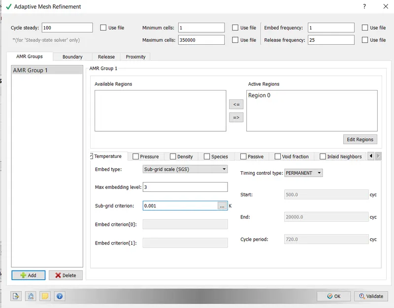
Adaptive Mesh Refinement :
In numerical analysis, adaptive Mesh refinement (AMR) is a method of adopting the accuracy of a solution with in certain sensitive and turbulence regions of simulation , dynamically and during the time the solution is being calculated numerically , they are often limited to per-determined quantified grids as in the Cartesian plane which constitute the computational Grid. Or mesh.Many Problems in numerical analysis , however do not require a uniform precision in the numerical grids used for graph plotting or computational simulations and would be better suited if specific areas of graphs which need precision could be refined in quantification only in the regions required the added precision. Adaptive mesh provides such a dynamic programming environment for adapting the precision of the numerical computation based on the requirements of a computational problems in specific areas of multidimensional graphs which need to precision while leaving of the multidimensional graphs at lower level of precision and resolution.
In our case we need more refined mesh at the shock were it could occur in that region we need more refinement of mesh in that area and the remaining should be the normal grid size mesh.
In converge we have the different methods which are used for the adaptive mesh refinement right now we are using the temp based sub grid criterion method with the two embedded layers . Thus the converge helps the curvature of temp property provided by AMR and starts he refining of the mesh for temp curvature by checking the values provided in SGS . This property helps us in the cost of computational domain and saves the time by not doing the unnecessary mesh for the entire domain.
In the Grid Control enable the AMR
Output and Post Processing:
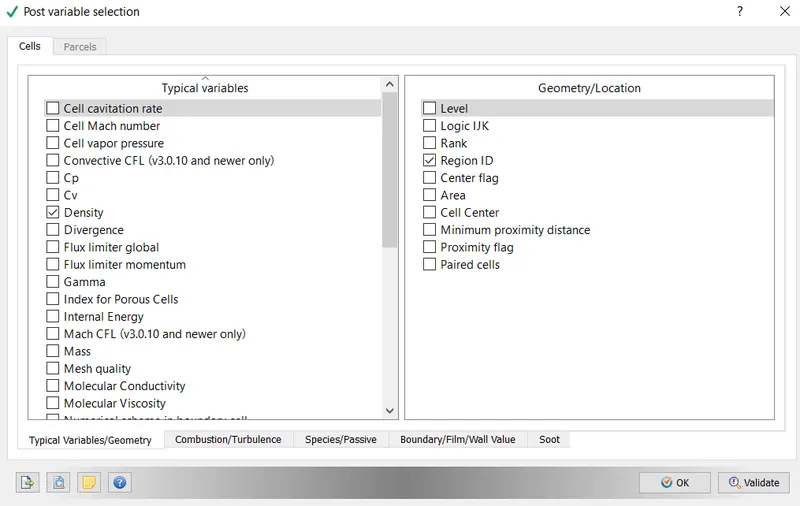
Post variable selection:
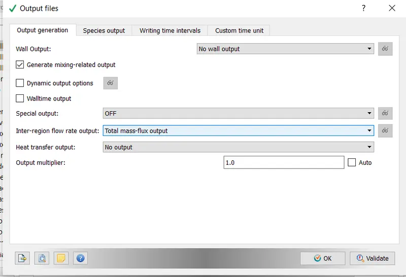
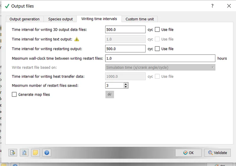
Output files:
Results:
To understand the Effect of SGS we have Performed Two setup's
Case1: SGS is 0.001 in AMR
Mesh:
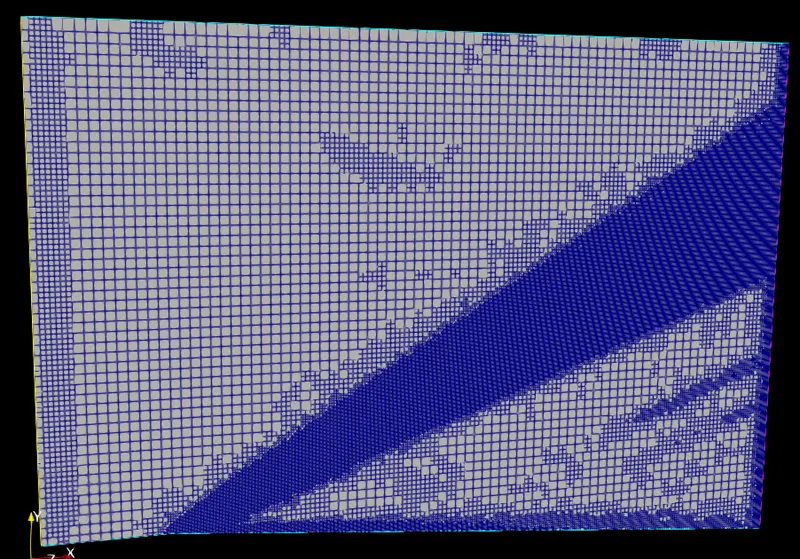
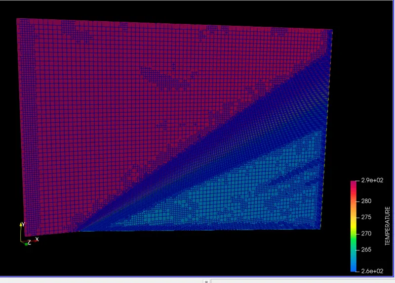
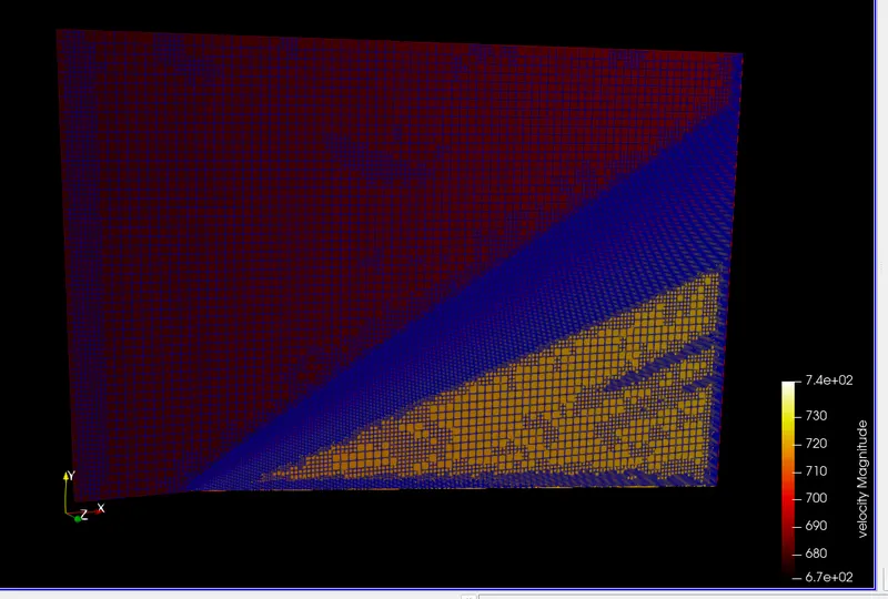
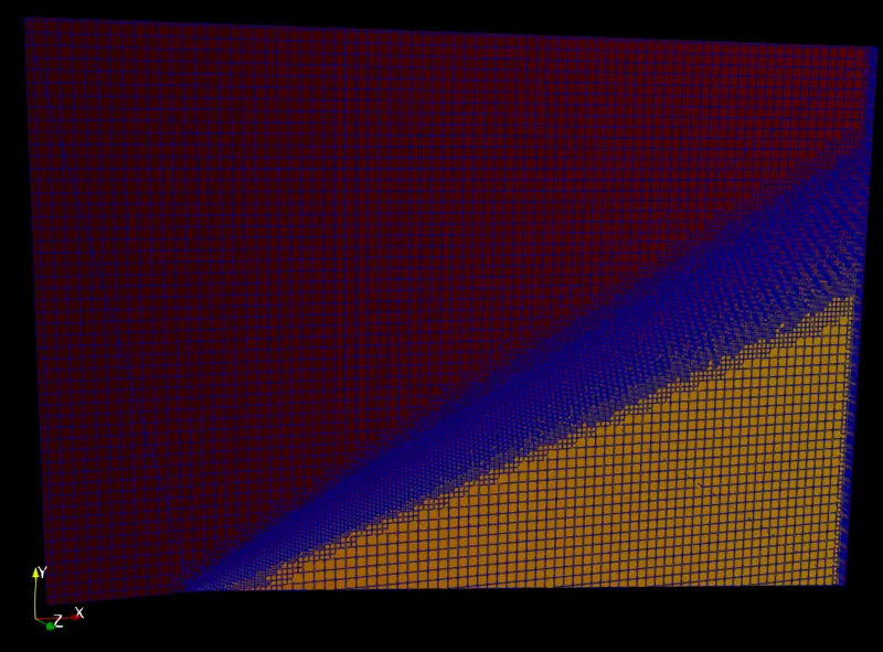
In the Mesh we can see that only the flow area the mesh is refined too good where we can see the Accuracy of flow.
Plot for Mach Number:
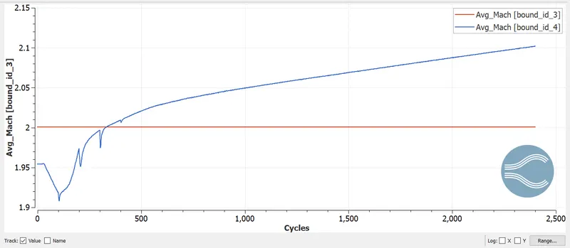
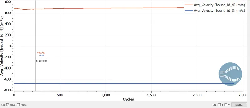
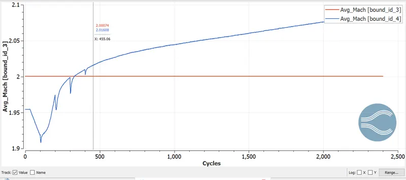
In mach plot due to the velocity 680m/s the speed of flow is seen as in graph 2.12 speed
Plot for Velocity:
Plot for Pressure:
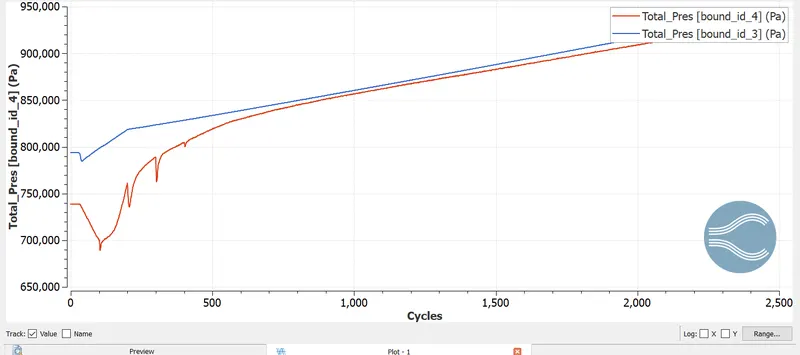
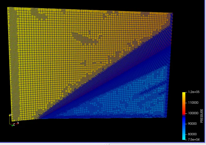
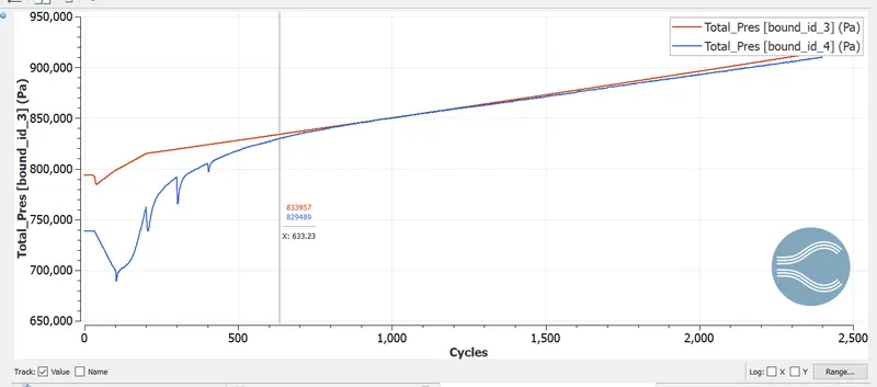
The pressure graph is shown the as the outlet as mentioned 101325 psi is mentioned and is increasing in graph
Plot for Temperature:
Plot for Cell count:
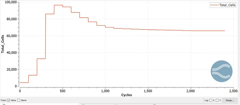
The cellc count 95000 is based on the 2450 cycles and the solution is reached to converge and the output is obtained.
Temperature Contour:
Velocity Contour:
Pressure contour:
Temperature Animation:
https://drive.google.com/file/d/1NbgHFxKq4C1y07KoJ52PWuKl7DbuYeDD/view?usp=sharing
Pressure Animation:
https://drive.google.com/file/d/1_9meZ01O9y43WvAagYRLsrSoLDMRFjGT/view?usp=sharing
Velocity Animation:
https://drive.google.com/file/d/1jUMwxcNG73Jblu416kE7phVyYYSV_bA4/view?usp=sharing
Case2: SGS is 0.01 in AMR
Mesh:
Plot for Mach Number:
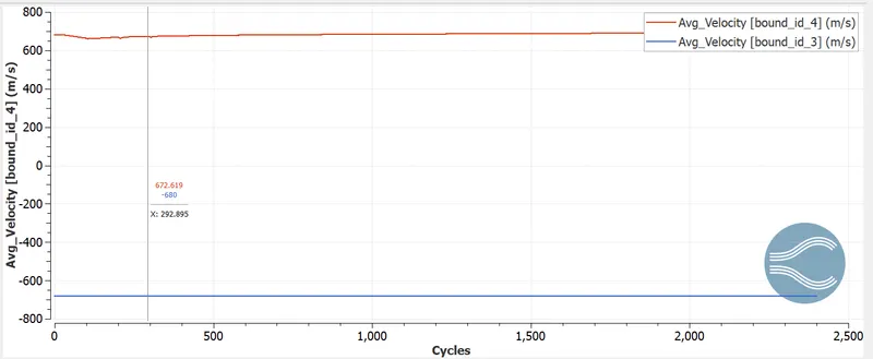
Plot for Velocity:
Plot for Pressure:
Plot for Temperature:
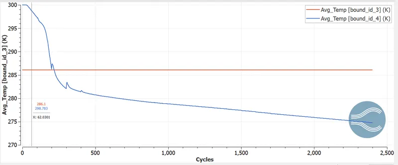
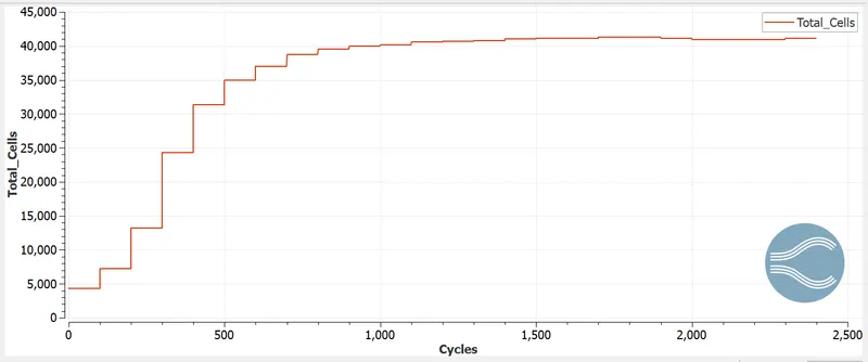
Plot for Cell count:
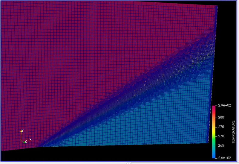
Temperature Contour:
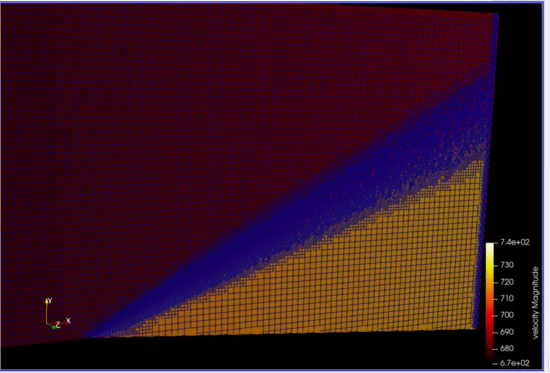
Velocity Contour:
Pressure contour:
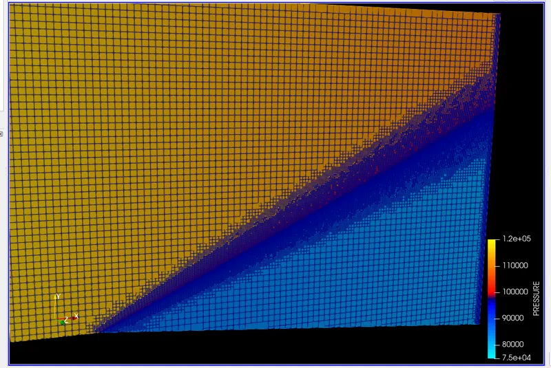
Temperature Animation:
https://drive.google.com/file/d/12O7c3jaUnVXmK8L1deQFaFLrugLkpVS4/view?usp=sharing
Pressure Animation:
https://drive.google.com/file/d/1napncauVUPqv5FsbI9Xo8kjr_HCZ1JnI/view?usp=sharing
Velocity Animation:
https://drive.google.com/file/d/1mzR8Fay4LgHAXqJq0Wb5uwrfc7-Drj2H/view?usp=sharing
Conclusion:
Two set of value of SGS are performed and observe the effects of sgs value in different parameters
We can clearly obseve with low value of SGS the fine mesh is observed
simulation of prandtl mayer number is done.
From the above plots we observe that the velocity increases the Mach increases and the pressure and temperature decreases