Week 5 - Mid term project - Solving the steady and unsteady 2D heat conduction problem

%%Steady state


clear all
close all
clc
ny=10;
nx=ny;
L=1;
dx=L/(nx-1);
dy=L/(ny-1);
x=linspace(0,L,nx);
y=linspace(0,L,ny);
k1=0.5*(dy^2/(dx^2+dy^2));
k2=0.5*(dx^2/(dx^2+dy^2));
%After applying the Boundary conditions
u=temperature_steady(nx,ny);
tol=1e-4;

%steady state Heat Conduction
iterative_solver=1;
if iterative_solver==1
  [u, jb_iter] =jacobi_method(u,tol,nx,ny,k1,k2);
  figure
  C=contourf(x,y,u,'edgecolor','none');
  clabel(C)
  colormap(jet)
  colorbar
  set(gca,'YDir','reverse')
end
if iterative_solver==2
    [u, gs_iter] =gs_method(u,tol,nx,ny,k1,k2);
     figure
  C=contourf(x,y,u,'edgecolor','none');
  clabel(C)
  colormap(jet)
  colorbar
  set(gca,'YDir','reverse')
end
if iterative_solver==3
    [u, sor_iter] =sor_method(u,tol,nx,ny,k1,k2);
     figure
  C=contourf(x,y,u,'edgecolor','none');
  clabel(C)
  colormap(jet)
  colorbar
  set(gca,'YDir','reverse')
end


Functions: 

Tmeperature matarix :
function out=temperature_steady(nx,ny)
   u=ones(nx,ny);
   %Applying BC to the system
   %T(top)=600k;T(bottom)=900k;T(right)=800k ; T(left)= 400
   %Consider Corner points to be average of adjacent points
   u(1)=500;
   u(nx*ny)=850;
   u((nx*(ny-1))+1)=700;
   u(nx)= 650;
   for i=2:(nx-1)
       u(i)=400;
   end
   for i=nx+1:nx:(nx-1)*(ny-1)
       u(i)=600;   
   end
   for i= 2*nx:nx:(nx*ny)-1
       u(i)=900;
   end
   for i=((nx-1)*ny)+2:((nx*ny)-1)
       u(i)=800;
   end
   out=u;
end
2) Jccobi Function :
function [out jb_iter] = jacobi_method(u,tol,nx,ny,k1,k2)
%Steady State Heat Transfer
   error=9e9;
   uold=u;
   jb_iter=1;
while(error>tol)
%Spatial loop 
   %x-loop
  for i=2:nx-1  
    % y-loop
      for j=2:ny-1
        u(i,j)=k1*(uold(i+1,j)+uold(i-1,j))+k2*(uold(i,j+1)+uold(i,j-1));
      end
  end
a=abs(uold-u);
error= max(a,[],'all');
uold=u;
jb_iter=jb_iter+1;
end
out=u;
end

3) Gauss-cidel Function :
function [out gs_iter] = gs_method(u,tol,nx,ny,k1,k2)
   error=9e9;
   uold=u;
   gs_iter=1;
while(error>tol)
%Spatial loop 
   %x-loop
  for i=2:nx-1  
    % y-loop
      for j=2:ny-1
        u(i,j)=k1*(uold(i+1,j)+u(i-1,j))+k2*(uold(i,j+1)+u(i,j-1));
      end
  end
a=abs(uold-u);
error= max(a,[],'all');
uold=u;
gs_iter=gs_iter+1;
end
out=u;
end
4)SOR METHOD:
function [out sor_iter] = sor_method(u,tol,nx,ny,k1,k2)
   error=9e9;
   uold=u;
   sor_iter=1;
   alpha=1.6;
while(error>tol)
%Spatial loop 
   %x-loop
  for i=2:nx-1  
    % y-loop
      for j=2:ny-1
        u(i,j)=(1-alpha)*uold(i,j)+alpha*(k1*(uold(i+1,j)+u(i-1,j))+k2*(uold(i,j+1)+u(i,j-1)));
        
      end
  end
a=abs(uold-u);
error= max(a,[],'all');
uold=u;
sor_iter=sor_iter+1;
end
out=u;
end 


%% TRANSIENT OR UNSTEADY STATE EQUATION

2D steady state equation

d²T/dx²+ d²T/dy² = 0

we need find the temperature at T_p i..e T_i,j

let

T_i-1,j= T_L

T_i+1,j= T_R

T_i,j-1= T_B

T_i,j+1= T_T

By Central differencing scheme we can write below equation as

d²T/dx²+ d²T/dy² = 0

(T_i+1,j-2T_i,j+T_i-1,j)/Δx² + (T_i,j+1-2T_i,j+T_i,j-1)/Δy² = 0

By above terminology and after arranging the terms we can deduce the equation to

2*T_p =( Δy²/ Δx²+ Δy²)(T_R+T_L) + ( Δx²/ Δx²+ Δy²)(T_T+T_B)

Let

0.5*(Δy²/ Δx²+ Δy²) = k₁

0.5*(Δx²/ Δx²+ Δy²)=k₂

T_p =k₁(T_R+T_L) + k₂ (T_T+T_B)…………… (1)

T_p =k₁(T_R +T_L) + k₂ (T_T+T_B)……..equation at the required point.

This can be solved by three process

1)Jacobi

2)Gauss-cidel

3)Sucessive over relaxation(SOR)

1)Jaccobi Method:

T_p =k₁(T_R +T_L) + k₂ (T_T+T_B) This equation is calculated at the nth time interval only T_p is at n+1 time interval.

So the above equation will be used in the program as

T_pⁿ⁺¹ = k₁ (T_i+1,jⁿ + T_i-1,jⁿ ) +k₂ (T_i,j+1ⁿ +T_i,j-1ⁿ )……………(2)

Where n – old time interval

N+1 – next time interval

2)Gauss-cidel Method:

T_p =k₁(T_R +T_L) + k₂ (T_T+T_B)

Known values in this equation are n time interval and unknown values are from n+1 .

So the above equation will be used in the program as

T_pⁿ⁺¹ = k₁ (T_i+1,jⁿ⁺¹ + T_i-1,jⁿ ) +k₂ (T_i,j+1ⁿ⁺¹ +T_i,j-1ⁿ )……………(3)

Where n – old time interval

N+1 – next time interval

3)SOR Method:

T_p =k₁(T_R +T_L) + k₂ (T_T+T_B)

α - SOR cofeeicient

SOR method is an enhancer for Jacobi or gauss cidel method

So the above equation will be used in the program as

T_pⁿ⁺¹ = 1-α(T_pⁿ) + α( k₁ (T_i+1,jⁿ⁺¹ + T_i-1,jⁿ ) +k₂ (T_i,j+1ⁿ⁺¹ +T_i,j-1ⁿ ))……………(4)

Gauss cidel solution

Where n – old time interval

N+1 – next time interval

Graphs :

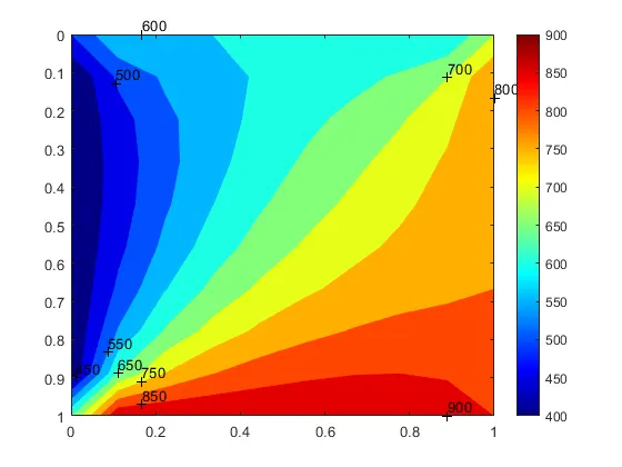
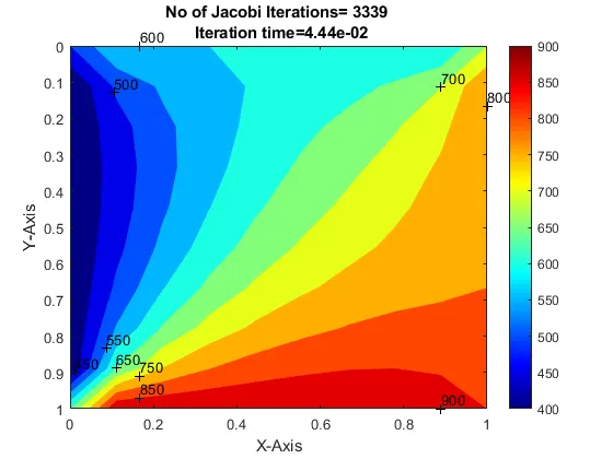
Jacobi Metehod:

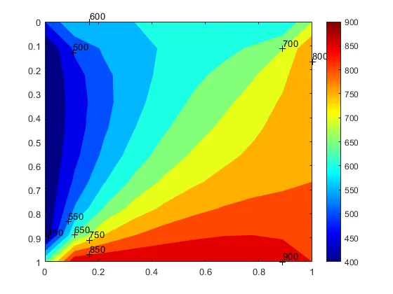
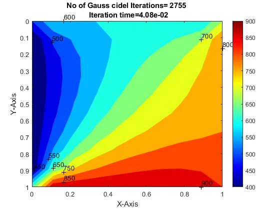
Guass-cidel Method:

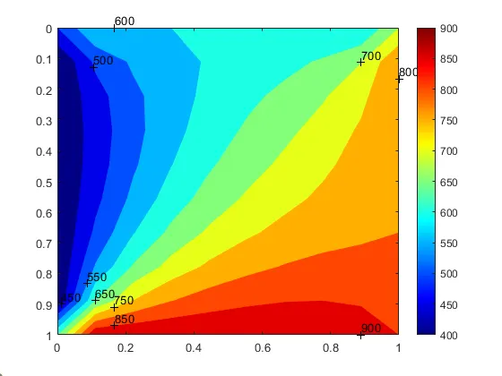
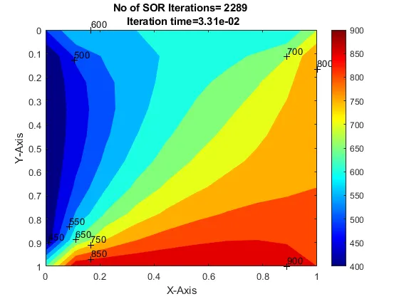
SOR Method:

Conclusions:

1)All the graphs from three methods looks similar but the number of iterations to achieve a steady solution varies.

2) Number of iterations to achieve the steady solution in Jacobi method is greater than gauss-cidel greater than SOR method.

Jacobi_iter>gs_iter>sor_iter

UnSteady State or Transient :

d²T/dt²+ α (d²T/dx²+ d²T/dy²) = 0

T_i,jⁿ⁺¹- T_i,jⁿ / Δt = α ((T_i+1,j-2T_i,j+T_i-1,j)/Δx² + (T_i,j+1-2T_i,j+T_i,j-1)/Δy²)

T_i-1,j= T_L

T_i+1,j= T_R

T_i,j-1= T_B

T_i,j+1= T_T

T_pⁿ⁺¹ = T_pⁿ + α Δt/ Δx² ( T_Rⁿ + T_Lⁿ)+ α Δt/ Δy² (T_T + T_B)-2* α*Δt*T_p(1/Δx²+1/Δy²)

Let α*Δt/Δx² = k1…………this is also called as CFL_X ……….(4)

α*Δt/Δy² = k₂ ………..this is also called as CFL_y………..(5)

let α = 1.5 for solids heat conduction.

To solve unsteady state equation we have to solve it time marching and also by the iterations. Time marching has two methods implicit and explicit methods.

We need to calculate the value of Δt by following equation

CFL ≤0.5………… (6)

CFL = CFL_x + CFL_y

K₁ +k₂ = 0.5 from eq 4,5 & 6

α*Δt/Δx² + α*Δt/Δy² = 0.5

by solving we will get Δt value.

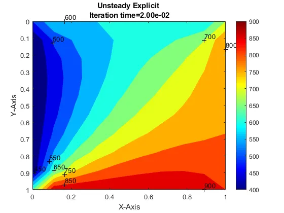
Explicit Method:

T_i,jⁿ⁺¹- T_i,jⁿ / Δt = [α ((T_i+1,j-2T_i,j+T_i-1,j)/Δx² + (T_i,j+1-2T_i,j+T_i,j-1)/Δy²)] ⁿ

Complete R.H.S term is calculated at n^th time interval.so final equation can be deduced to

T_pⁿ⁺¹ = T_pⁿ [1-2k₁-2k₂] + k₁[ T_R+T_L]ⁿ + k₂[T_T+T_B]ⁿ

^Graph:

Implicit Method:

T_i,jⁿ⁺¹- T_i,jⁿ / Δt = [α ((T_i+1,j-2T_i,j+T_i-1,j)/Δx² + (T_i,j+1-2T_i,j+T_i,j-1)/Δy²)] ⁿ⁺¹

Complete R.H.S term is calculated at n+1^th time interval.so final equation can be deduced to

T_pⁿ⁺¹=[T_pⁿ +k₁(T_R+T_L )ⁿ⁺¹ +k₂ (T_T+T_B)ⁿ⁺¹ ] /(1+2k₁+2k₂)……………

1)Jaccobi Method:

T_pⁿ⁺¹=[T_pⁿ +k₁(T_R+T_L )ⁿ⁺¹ +k₂ (T_T+T_B)ⁿ⁺¹ ] /(1+2k₁+2k₂) This equation is calculated at the nth time interval , only T_p at L.H.S is at n+1 time interval.

So the above equation will be used in the program as

T_pⁿ⁺¹ = k₁ (T_i+1,jⁿ + T_i-1,jⁿ ) +k₂ (T_i,j+1ⁿ +T_i,j-1ⁿ )……………(2)

Where n – old time interval

N+1 – next time interval

2)Gauss-cidel Method:

T_pⁿ⁺¹=[T_pⁿ +k₁(T_R+T_L )ⁿ⁺¹ +k₂ (T_T+T_B)ⁿ⁺¹ ] /(1+2k₁+2k₂) ] above equation can be deduced to

T_pⁿ⁺¹ = T_pⁿ *1/(1+2k₁+2k₂) +k1/(1+2k₁+2k₂) *(T_Lⁿ⁺¹ +T_Rⁿ)+ k2/(1+2k₁+2k₂) * (T_Tⁿ⁺¹ + T_Bⁿ)

Where in coding we can designate as

1/(1+2k₁+2k₂) = term1

k1/(1+2k₁+2k₂) =term2

k2/(1+2k₁+2k₂)= term3

final equation is

T_pⁿ⁺¹ = term1*T_pⁿ + term2* (T_Lⁿ⁺¹ + T_Rⁿ)+ term3*(T_Tⁿ⁺¹ + T_Bⁿ)

Where n – old time interval

N+1 – next time interval

3)SOR Method :

T_pⁿ⁺¹=[T_pⁿ +k₁(T_R+T_L )ⁿ⁺¹ +k₂ (T_T+T_B)ⁿ⁺¹ ] /(1+2k₁+2k₂) ] above equation can be deduced to

α - SOR coefficient

SOR method is an enhancer for Jacobi or gauss cidel method

So the above equation will be used in the program as

T_pⁿ⁺¹ = 1-α(T_pⁿ) + α(T_pⁿ *1/(1+2k₁+2k₂) +k1/(1+2k₁+2k₂) *(T_Lⁿ⁺¹ +T_Rⁿ)+ k2/(1+2k₁+2k₂) * (T_Tⁿ⁺¹ + T_Bⁿ) )……………(3)

final equation is

T_pⁿ⁺¹ = 1-α(T_pⁿ) + α (term1*T_pⁿ + term2* (T_Lⁿ⁺¹ + T_Rⁿ)+ term3*(T_Tⁿ⁺¹ + T_Bⁿ)

Where n – old time interval

N+1 – next time interval

Graph:

Conclusions:

1)Solving the function in explicit has more iterations than solving the equation in implicit method.

2)All the graphs from three methods looks similar but the number of iterations to achieve a steady solution varies.

3) Number of iterations to achieve the steady solution in Jacobi method is greater than gauss-cidel greater than SOR method.

Jacobi_iter>gs_iter>sor_iter