Week 5 - Mid term project - Solving the steady and unsteady 2D heat conduction problem

AIM:

To solve the Steady and Unsteady state 2D Heat Conduction problem by using point iterative techniques for both Implicit and Explicit techniques using MATLAB.

Problem Statement:

1. The domain length is assumed to be unit square.
2. Assumption nx =ny, i.e. no of grid points on both x and y-axis should be equal.
3. Assumed nx=ny=10.
4. Boundary conditions are

Left=400K

Right=800K

Top=600K

Bottom=900K

5. Let the initial temperature be 300K.
6. Using Steady and Unsteady state condition, solve the equation
7. We have to find no of iterations each solver takes to solve the equation.

There are various schemes for solving implicit equations.

1. Jacobi
2. Gauss-Seidel

• Successive over-relaxation (SOR)

THEORY:

The heat equation is a partial differential equation that describes how the distribution of heat evolves over time. For a function u (x, y, z, t) of the three spatial variables (x, y, z) i.e. Cartesian coordinate system and the time variable t, hence the heat equation is

`\frac{\partial u}{\partial t}=\alpha(\frac{\partial^2u}{{\partial x}^2}+\frac{\partial^2u}{{\partial y}^2}+\frac{\partial^2u}{{\partial z}^2})`

Where,

`\alpha\ is\ thermal\ diffusivity`

The good initial condition will lead to converging steady-state conditions faster. So, the assumed value is 300K, when the solution gets converge then it is washed out.

IMPLICIT Schemes (Steady State Condition)

Steady-State Equation 2D Heat Conduction

In steady-state conduction, the amount of heat entering the region is equal to the amount of heat coming out.

Steady-state 2D heat conduction equation is as follows

`\frac{\partial^2T}{{\partial x}^2}+\frac{\partial^2T}{{\partial y}^2}=0`

Nomenclature

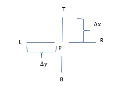
`∆x`- the distance between points L and P

`∆y`- the distance between point T and P

On discretizing the equation

`T_p=\frac{1}{K}(TL+TR∆x2)+\ \frac{1}{K}(TT+TB∆y2)`

`T_p=\frac{1}{K}TL+TR∆x2+TT+TB∆y2`

Where `K=2∆x2+∆y2∆x2∆y2`

Now we have an equation for the temperature at point P. Then we will use iterative techniques like Jacobi, Gauss seidel, and SOR to compute the value of `T_p.`

On further simplification the equation is

`0.25*(T_L+T_R+T_T+T_B)`

In cartesian form it can be written as

`T_{i,j}=0.25(T_{old(i-1,j)}+T_{old(i+1,j)}+T_{old(i,j-1)}+T_{old(i,j+1)})`

GAUSS-SEIDEL

The equation for Gauss-Seidel is

`T_{i,j}=0.25(T_{(i-1,j)}+T_{old(i+1,j)}+T_{(i,j-1)}+T_{old(i,j+1)}`

SUCCESSIVE OVER REALAXATIO(SOR)

The final equation for SOR is

`T_{i,j}=(1-\omega)T_{old}+\omega(0.25(T_{(i-1,j)}+T_{old(i+1,j)}+T_{(i,j-1)}+T_{old(i,j+1)})`

Where,

`\omega=Realxation\ factor`

`If \omega > 1, over relaxation`

`\omega <1, under relaxation`

Here, we have kept `\omega` value between to 1.1-1.2

% solve the 2D heat conduction equation by using the point iterative
% techniques
clear all
close all
clc
L=1;% Domain Length
% No of grid points
nx=10;
ny=nx;
% Grid Spacing
x=linspace(0,L,nx);
dx=x(2)-x(1);  % for finding the K value dx is required
% Similarly dy is also required 
y=x;
dy=y(2)-y(1);
% Boundary Conditions
T=ones(nx,ny);
T(:,1)=400;  % all the elements in the first column will be 400
T(1,:)=600; % all the elements in the first row will be 600
T(:,end)=800; % all the elements in the last column will be 800
T(end,:)=900; % all the elemnts in the last row will be 900
T(1,1)=0.5*(T(1,2)+T(2,1));% Top left corner temperature
T(end,1)=0.5*(T(end-1,1)+T(end,2));% Bottom left corner temperature
T(end,end)=0.5*(T(end,end-1)+T(end-1,end));% Bottom right corner temperature
T(1,end)=0.5*(T(1,end-1)+T(2,end));% Top right corner temperature
Told=T;  % We have to even define Told value
% Absolute error
error=9e9;
tol=1e-4;
iterative_solver=input;%% Input can be 1,2,or 3 according to the required iterative
 %% Jacobi Method
 if iterative_solver==1
     jacobi_iter=1;
     while (error>tol)
         for i=2:nx-1
             for j=2:ny-1
                 T(i,j)=0.25*(Told(i-1,j)+Told(i+1,j)+Told(i,j+1)+Told(i,j-1)); % K=0.25 calculated by the formula
             end
         end
         error_n=max(abs(Told-T));
         error=max(error_n);
         
         Told=T;  % To update the old T Values
         [C,h]=contourf(x,y,T);
         clabel(C,h,'Fontsize',8);
         colorbar
         jacobi_iter=jacobi_iter+1;
         title_text=sprintf('Jacobi Iteration Number=%d',jacobi_iter);
         title(title_text);
         pause(0.03)
     end
 end
%% Gauss Siedel Method

  if iterative_solver==2
     gs_iter=1;
     while (error>tol)
         for i=2:nx-1
             for j=2:ny-1
                 T(i,j)=0.25*(T(i-1,j)+T(i+1,j)+T(i,j+1)+T(i,j-1)); % K=0.25 calculated by the formula
             end
         end
         error_n=max(abs(Told-T));
         error=max(error_n);
         
         Told=T;  % To update the old T Values
         [C,h]=contourf(x,y,T);
         clabel(C,h,'Fontsize',8);
         colorbar
         gs_iter=gs_iter+1;
         title_text=sprintf('Gauss Siedel Iteration Number=%d',gs_iter);
         title(title_text);
         pause(0.03)
     end
 end
%% Successive Over Relaxation (sor)

 if iterative_solver==3
     sor_iter=1;
     w=1.9; % w(omega)(relaxation factor for sor)
     while (error>tol)
         for i=2:nx-1
             for j=2:ny-1
                 T(i,j)=(1-w)*Told(i,j)+w*(0.25*(T(i-1,j)+T(i+1,j)+T(i,j+1)+T(i,j-1))); % K=0.25 calculated by the formula
             end
         end
         error_n=max(abs(Told-T));
         error=max(error_n);
         
         Told=T;  % To update the old T Values
         [C,h]=contourf(x,y,T);
         clabel(C,h,'Fontsize',8);
         colorbar;
         sor_iter=sor_iter+1;
         title_text=sprintf('SOR Iteration Number=%d',sor_iter);
         title(title_text);
         pause(0.03)
     end
 end

Plots and Results:

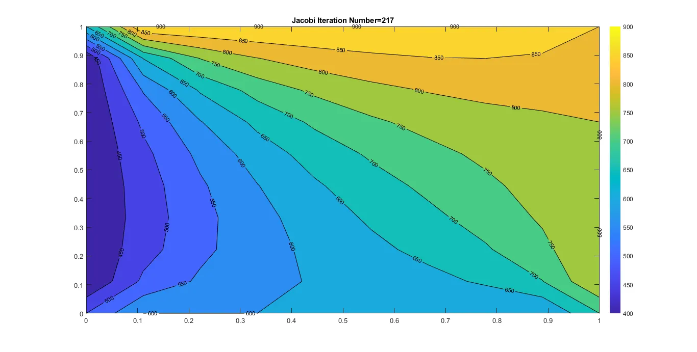
1. Jacobi Method
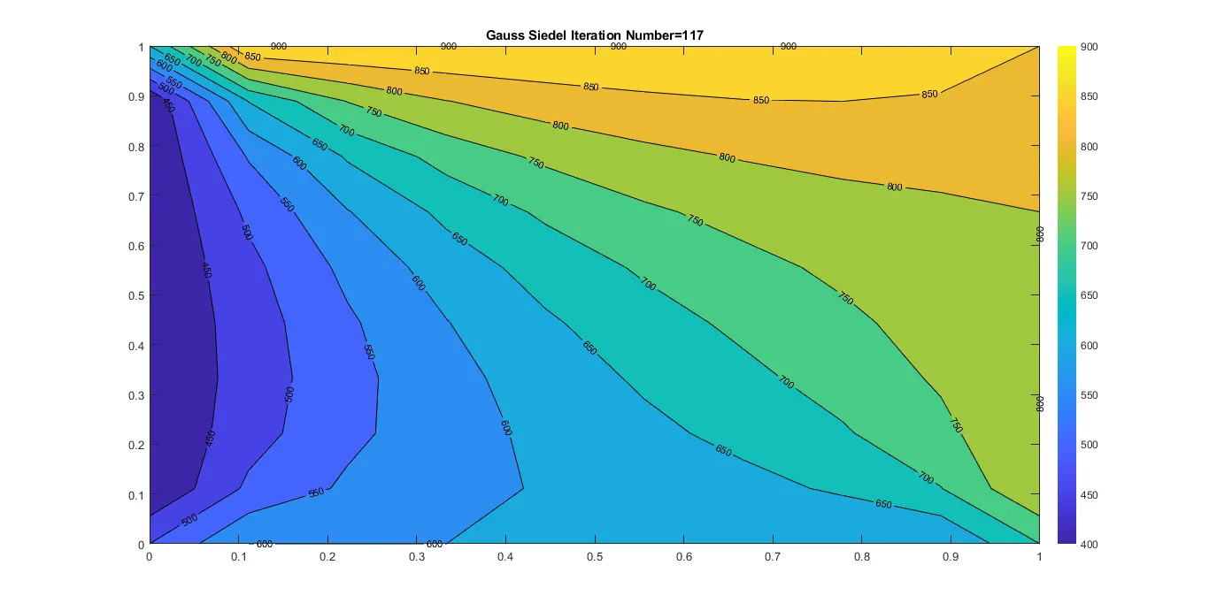
2. Gauss-Seidel Method(GS)
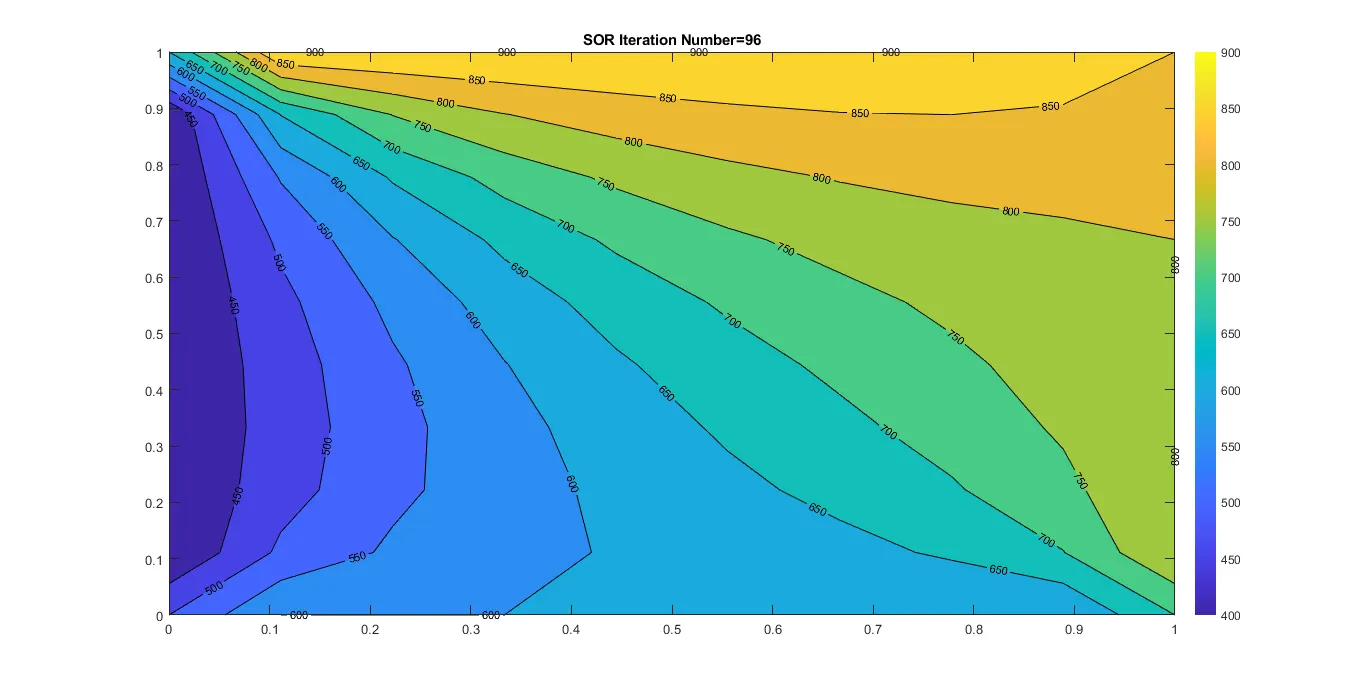
3. SOR(ω=1.1)
4. SOR(ω=1.9)

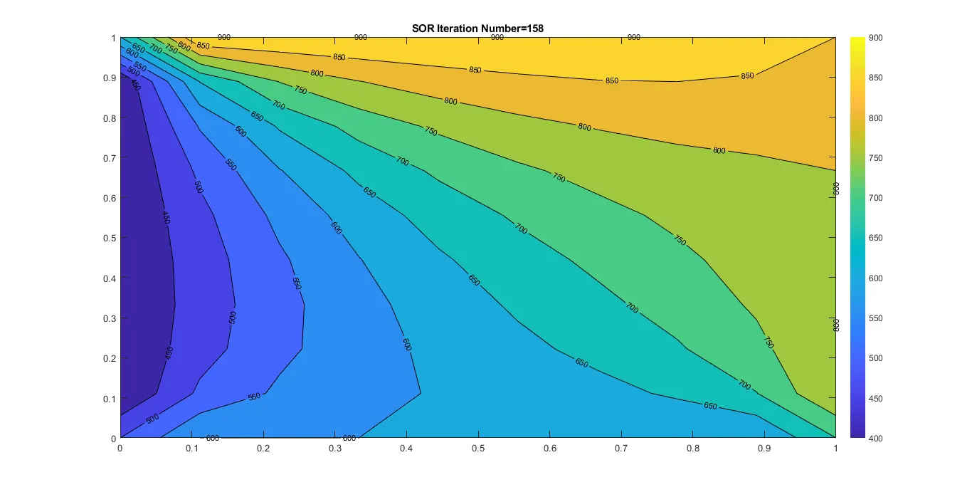
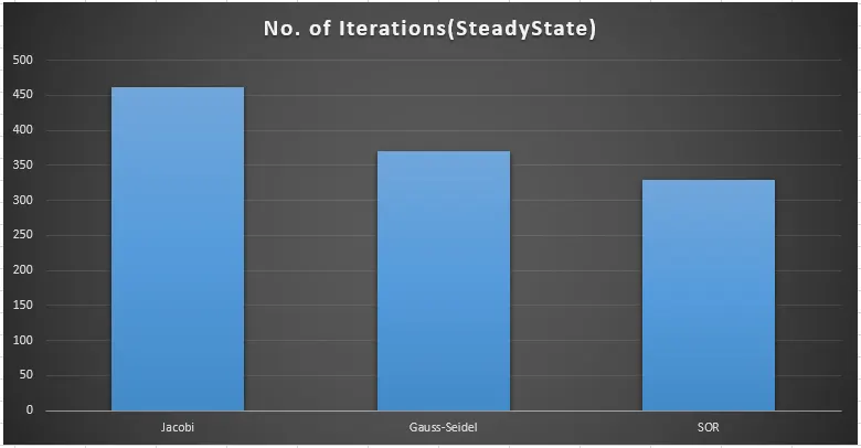
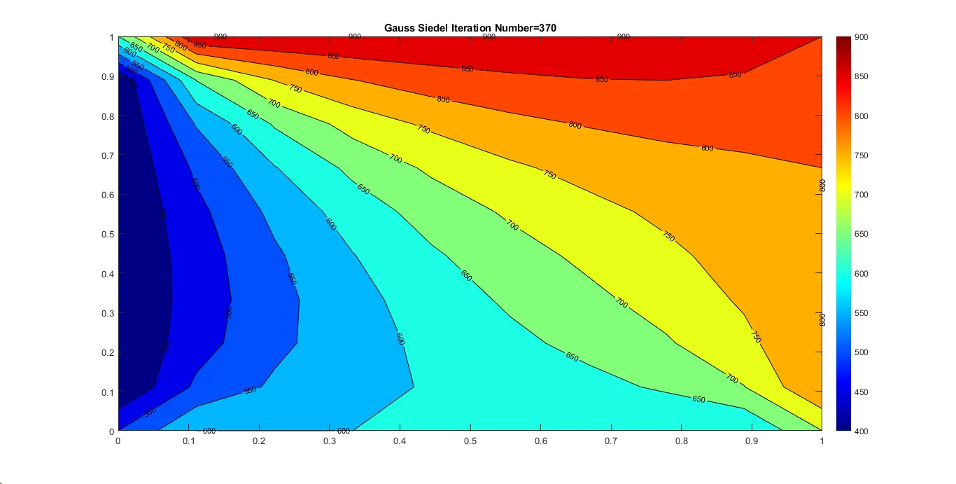
On comparing the three iterative techniques it was found that the computational time required to converge the solution was highest in the Jacobi Method as it doesn’t update its values and continues with the guess value. Whereas the Gauss-Seidel Method, it uses the updated value of the previous iteration the no of iterations required to converge the solution is less in the SOR Method due to the use of a relaxation factor. If, the alpha >1, then it is called over relaxation and the solution gets converge faster. If the correction factor is higher than required, then the solution can blow instead of converging and the solution diverges.

UNSTEADY STATE/TRANSIENT STATE

The general equation

`\frac{\partial T}{\partial t}=\alpha(\frac{\partial^2T}{{\partial x}^2}+\frac{\partial^2T}{{\partial y}^2})`

Nomenclature

`T_p^{n+1}`

- Next time step

`T_p^n-\ Present\ time\ step`

Hence the equation is

`Tpn+1-Tpn∆t=αTL-2TP+TR∆x2+TT-2TP+TR∆y2`

`Tpn+1-Tpn∆t=αTL-2TP+TR∆x2+TT-2TP+TR∆y2n or n+1`

If n-Explicit

n+1- Implicit

For Explicit

`Tpn+1-Tpn∆t=αTL-2TP+TR∆x2+TT-2TP+TR∆y2n`

Hence on solving we get

`T_p^{n+1}=T_p^n+K_1(T_L-2T_P+T_R)+K_2(T_T-2T_P+T_B)`

where,

`K1=\ \alpha∆T∆x2`

`K2=\ \alpha∆T∆y2`

`T_{i,j}=term1+term2+term3`

Where,

`Term1-T_p^n`

`Term2-K_1(T_L-2T_P+T_R)`

`Term3-K_2(T_T-2T_P+T_B)`

%Unsteady state 2D heat conductionusing explicit method
clear all
close all
clc
L=1;% Domain Length
% No of grid points
nx=10;
ny=nx;
n=200;
% Grid Spacing
x=linspace(0,L,nx);
dx=x(2)-x(1);  % for finding the K value dx is required
% Similarly dy is also required 
y=x;
dy=y(2)-y(1);
% Boundary Conditions
T=ones(nx,ny);
T(:,1)=400;  % all the elements in the first column will be 400
T(1,:)=600; % all the elements in the first row will be 600
T(:,end)=800; % all the elements in the last column will be 800
T(end,:)=900; % all the elemnts in the last row will be 900
T(1,1)=0.5*(T(1,2)+T(2,1));% Top left corner temperature
T(end,1)=0.5*(T(end-1,1)+T(end,2));% Bottom left corner temperature
T(end,end)=0.5*(T(end,end-1)+T(end-1,end));% Bottom right corner temperature
T(1,end)=0.5*(T(1,end-1)+T(2,end));% Top right corner temperature
Told=T;  % Previous temperature
dt=0.01; %it is required to find the k values
% thermal diffusivity
alpha=0.25; % assumed value
%% Now applying the formulae
k1=alpha*(dt/dx^2);
k2=alpha*(dt/dy^2);
iterative=1;
%%Time loop
for nt=1:n
    for i=2:nx-1
        for j=2:ny-1
            term1=Told(i,j);
            term2=k1*(T(i-1,j)-2*Told(i,j)+T(i+1,j));
            term3=k1*(T(i,j-1)-2*Told(i,j)+T(i,j+1));
            T(i,j)=term1+term2+term3; % According to the expression
        end
    end
    Told=T; % update the temperature
    colormap(jet)
    [C,h]=contourf(x,y,T);
    clabel(C,h);
    colorbar;
    title_text=sprintf('No of iteration=%d',iterative);
    title(title_text);
    iterative=iterative+1;
    pause(0.03);
    
end

For Implicit

`Tpn+1-Tpn∆t=αTL-2TP+TR∆x2+TT-2TP+TR∆y2n+1`

`T_p^{n+1}=\frac{1}{1+2K1+2K2}\left\lfloor T_p^n+{K_1(T_L+T_R)}^{n+1}+{K_2(T_T+T_B)}^{n+1}\right\rfloor`

`K_1- \alpha\frac{\Delta t}{\Delta x^2}`

`K_2- \alpha\frac{\Delta t}{\Delta y^2}`

`Term1=\frac{1}{1+2K1+2K2}`

`Term2=K_1* term`

`Term3=K_2* term1`

Hence the equation becomes

`T_p^{n+1}=term1xT_p^n+term2x{(T_L+T_R)}^{n+1}+term3x{(T_T+T_B)}^{n+1}`

We cannot solve the equation directly as there are many unknowns. So, we will go for iterative methods, I.e. Jacobi, Gauss-Seidel, SOR to solve for the temperature.

%Unsteady state 2D heat conductionusing implicit method
clear all
close all
clc
L=1;% Domain Length
% No of grid points
nx=10;
ny=nx;
n=200;
% Grid Spacing
x=linspace(0,L,nx);
dx=x(2)-x(1);  % for finding the K value dx is required
% Similarly dy is also required 
y=x;
dy=y(2)-y(1);
% Boundary Conditions
T=ones(nx,ny);
T(:,1)=400;  % all the elements in the first column will be 400
T(1,:)=600; % all the elements in the first row will be 600
T(:,end)=800; % all the elements in the last column will be 800
T(end,:)=900; % all the elemnts in the last row will be 900
T(1,1)=0.5*(T(1,2)+T(2,1));% Top left corner temperature
T(end,1)=0.5*(T(end-1,1)+T(end,2));% Bottom left corner temperature
T(end,end)=0.5*(T(end,end-1)+T(end-1,end));% Bottom right corner temperature
T(1,end)=0.5*(T(1,end-1)+T(2,end));% Top right corner temperature
Told=T;  % Previous temperature
dt=0.01; %it is required to find the k values
% thermal diffusivity
alpha=0.25; % assumed value
w=1.9;
%% Now applying the formulae
k1=alpha*(dt/dx^2);
k2=alpha*(dt/dy^2);
z=1;
error=9e9;
tol=1e-4;
iterative_solver=3;
%% Jacobi Method
%Time loop
for nt=1:n
    if iterative_solver==1
        jacobi_iter=1;
        while error>tol
            for i=2:nx-1
                for j=2:ny-1
                    term1=(1/(1+2*k1+2*k2));
                    term2=k1*term1;
                    term3=k2*term1;
                    TL=Told(i-1,j);% temperature on the left side
                    TR=Told(i+1,j);% temperature on the rightt side
                    TT=Told(i,j-1);% temperature on the top side
                    TB=Told(i,j+1);% temperature on the bottom side
                    T(i,j)=(term1*Told(i,j))+(term2*(TL+TR))+(term3*(TT+TB));
                end
            end
            error_n=max(abs(Told-T));
            error=max(error_n);
            Told=T;
            colormap(jet)
            [C,h]=contourf(x,y,T);
            clabel(C,h,'Fontsize',8);
            jacobi_iter=jacobi_iter+1;
            title_text=sprintf('Jacobi Iteration Number=%d',jacobi_iter);
            title(title_text)
            colorbar
            pause(0.03)
        end
    end
    
end
%% Gauss Siedel Method
%Time loop
for nt=1:n
    if iterative_solver==2
        gs_iter=1;
        while error>tol
            for i=2:nx-1
                for j=2:ny-1
                    term1=(1/(1+2*k1+2*k2));
                    term2=k1*term1;
                    term3=k2*term1;
                    TL=T(i-1,j);% temperature on the left side
                    TR=Told(i+1,j);% temperature on the rightt side
                    TT=T(i,j-1);% temperature on the top side
                    TB=Told(i,j+1);% temperature on the bottom side
                    T(i,j)=(term1*Told(i,j))+(term2*(TL+TR))+(term3*(TT+TB));
                end
            end
            error_n=max(abs(Told-T));
            error=max(error_n);
            Told=T;
            colormap(jet)
            [C,h]=contourf(x,y,T);
            clabel(C,h,'Fontsize',8);
            gs_iter=gs_iter+1;
            title_text=sprintf('Gauss Siedel Iteration Number=%d',gs_iter);
            title(title_text)
            colorbar
            pause(0.03)
        end
    end
    
end                    
%% Successive over Relaxation Method
%Time loop
for nt=1:n
    if iterative_solver==3
        sor_iter=1;
               while error>tol
            for i=2:nx-1
                for j=2:ny-1
                    term1=(1/(1+2*k1+2*k2));
                    term2=k1*term1;
                    term3=k2*term1;
                    TL=T(i-1,j);% temperature on the left side
                    TR=Told(i+1,j);% temperature on the rightt side
                    TT=T(i,j-1);% temperature on the top side
                    TB=Told(i,j+1);% temperature on the bottom side
                    T(i,j)=(1-w)*Told(i,j)+w*((term1*Told(i,j))+(term2*(TL+TR))+(term3*(TT+TB)));
                end
            end
            error_n=max(abs(Told-T));
            error=max(error_n);
            Told=T;
            colormap(jet)
            [C,h]=contourf(x,y,T);
            clabel(C,h,'Fontsize',8);
            sor_iter=sor_iter+1;
            title_text=sprintf('SOR Iteration Number=%d',sor_iter);
            title(title_text)
            colorbar
            pause(0.03)
        end
    end
    
end                    

PLOTS AND RESULTS:

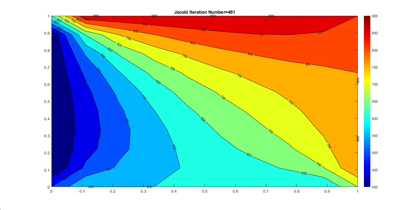
1. Jacobi
2. Gauss-Seidel Method
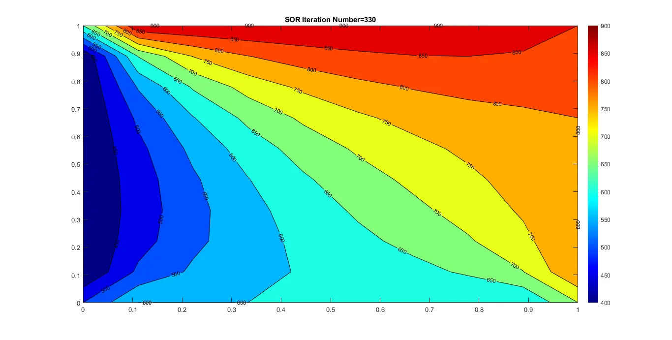
3. SOR(ω=1.1)
4. SOR(ω=1.9)

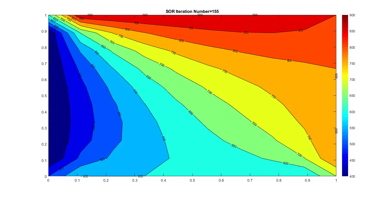
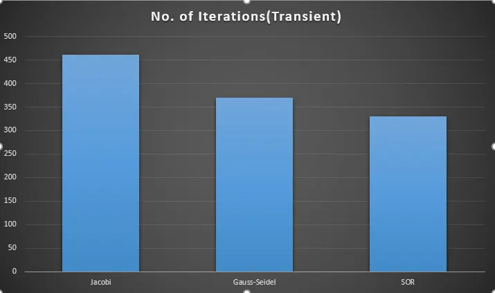
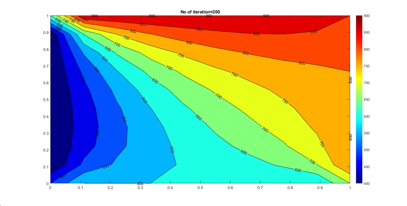
The transient analysis gives better performance compared to the steady-state as it depicts the real-world scenario. The transient analysis takes into consideration the varying rate of heat transfer with respect to time.

Similar to steady-state analysis, the no of iterations required to converge the solution was falling from the Jacobi method to the SOR Method as depicted by the bar graph.