Week 5 - Mid term project - Solving the steady and unsteady 2D heat conduction problem
AIM :
To solve the 2D heat conduction equation by using the point iterative techniques.
ie Jacobi Method
Gauss Seidel Method
Successive Over relaxation Method
BOUNDARY CONDITIONS:
The region is a square domain where nx = ny
Top Boundary = 600 K
Bottom Boundary = 900 K
Left Boundary = 400 K
Right Boundary = 800 K
DEDUCTION:
The values given above are generic for the region. To know the specific values of temperature at the corners, we need to take average of the subsequent boundaries and arrive at a particular temperature..
Top Left: (Top Boundary + Left Boundary) / 2
Bottom Left: (Bottom Boundary + Left Boundary) / 2
Top Right: (Top Boundary + Right Boundary) / 2
Bottom Left: (Bottom Boundary + Left Boundary) / 2
NOTE: We assume an equivalent or initial temperature of 300k at all nodal points.
STEADY STATE THEORY:
A stable condition that does not change over time or in which change in one direction is continually balanced by change in another.
The 2D heat conduction equation is given below..
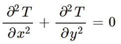
The main purpose is to solve is equation at differnent states as per the given boundary conditions..
To solve a equation, we have to discretize it first in CFD..
So discretizing this equation by taking values from the (point above , below, left and right) surrounding points , we get
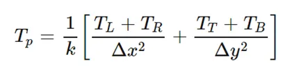
Where
Tp is the given point
Δx is the difference between two points in x axis
Δy is the difference between two points in y axis
K = 2 (Δx2 + Δy2)/( Δx Δy)
The final equation breaks down to,

PROGRAM CODE FOR STEADY STATE - JACOBI METHOD:
clear all
close all
clc
L = 1 ;
nx = 10 ;
ny = 10;
x = linspace(0,1,nx)
y = linspace(0,1,ny)
dx = x(2) - x(1) ;
dy = dx ;
t = 300*ones(nx,ny);
% Boundary Conditions
t(2:ny-1,1) = 400;
t(2:ny-1,nx)= 800;
t(1,2:nx-1) = 600;
t(ny,2:nx-1) = 900;
t(1,1) = 500
t(1,ny) = 700
t(nx,1) = 650
t(nx,ny) = 850
t_initial=t;
told = t ;
error = 9e9;
tolerance = 1e-4;
iterative_solver = 1 ;
if iterative_solver == 1
jacobi_iteration = 1 ;
while( error > tolerance)
for i= 2:nx-1
for j=2:ny-1
t(i,j) = 0.25*((told(i-1,j)) + (told(i+1,j)) + (told(i,j-1)) + (told(i,j+1)));
end
end
error = max(max(abs(told - t)))
told = t
jacobi_iteration = jacobi_iteration +1 ;
end
end
figure(1)
contour(x,y,t)
clabel(contour(x,y,t))
colorbar
colormap(jet)
set(gca,'ydir','reverse')
xlabel('x axis')
ylabel('y axis')
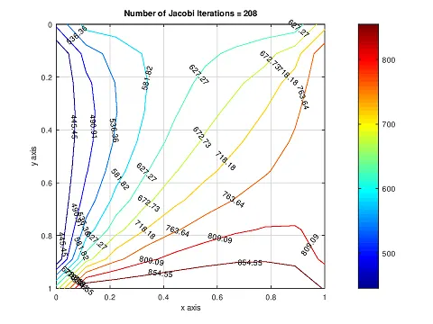
title(sprintf('Number of Jacobi Iterations = %d',jacobi_iteration));
pause(0.03);
PLOT :
PROGRAM CODE FOR STEADY STATE - GAUSS SEIDEL METHOD:
clear all
close all
clc
L = 1 ;
nx = 10 ;
ny = 10;
x = linspace(0,1,nx)
y = linspace(0,1,ny)
dx = x(2) - x(1) ;
dy = dx ;
t = 300*ones(nx,ny);
% Boundary Conditions
t(2:ny-1,1) = 400;
t(2:ny-1,nx)= 800;
t(1,2:nx-1) = 600;
t(ny,2:nx-1) = 900;
t(1,1) = 500
t(1,ny) = 700
t(nx,1) = 650
t(nx,ny) = 850
t_initial=t;
told = t ;
error = 9e9;
tolerance = 1e-4;
iterative_solver = 2 ;
if iterative_solver == 2
GS_iteration = 1 ;
while( error > tolerance)
for i= 2:nx-1
for j=2:ny-1
t(i,j) = 0.25*((t(i-1,j)) + (told(i+1,j)) + (t(i,j-1)) + (told(i,j+1)));
end
end
error = max(max(abs(told - t)))
told = t
GS_iteration = GS_iteration +1 ;
end
end
figure(1)
contour(x,y,t)
clabel(contour(x,y,t))
colorbar
colormap(jet)
set(gca,'ydir','reverse')
xlabel('x axis')
ylabel('y axis')
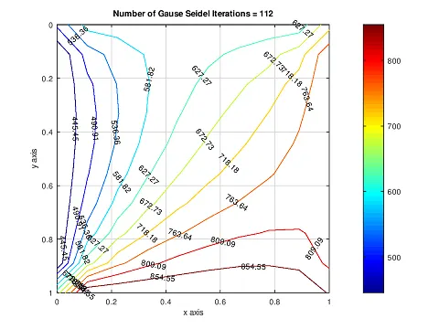
title(sprintf('Number of Gause Seidel Iterations = %d',GS_iteration));
pause(0.03);
PLOT:
PROGRAM CODE FOR STEADY STATE - SUCCESSIVE OVER RELAXATION METHOD
clear all
close all
clc
L = 1 ;
nx = 10 ;
ny = 10;
x = linspace(0,1,nx);
y = linspace(0,1,ny);
dx = x(2) - x(1) ;
dy = dx ;
t = 300*ones(nx,ny);
% Boundary Conditions
t(2:ny-1,1) = 400;
t(2:ny-1,nx)= 800;
t(1,2:nx-1) = 600;
t(ny,2:nx-1) = 900;
t(1,1) = 500;
t(1,ny) = 700;
t(nx,1) = 650;
t(nx,ny) = 850;
t_initial=t;
told = t ;
error = 9e9;
tolerance = 1e-4;
omega = 1.4;
iterative_solver = 3 ;
if iterative_solver == 3
SOR_iteration = 1 ;
while( error > tolerance)
for i= 2:nx-1
for j=2:ny-1
t(i,j) = omega*(0.25*((t(i-1,j)) + (told(i+1,j)) + (t(i,j-1)) + (told(i,j+1)))) + (1-omega) * told(i,j);
end
end
error = max(max(abs(told - t)));
told = t;
SOR_iteration = SOR_iteration +1 ;
end
end
figure(1)
contour(x,y,t)
clabel(contour(x,y,t))
colorbar
colormap(jet)
set(gca,'ydir','reverse')
xlabel('x axis')
ylabel('y axis')
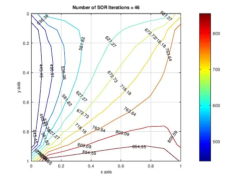
title(sprintf('Number of SOR Iterations = %d',SOR_iteration));
pause(0.03);
PLOT :
UNSTEADY STATE THEORY- EXPLICIT METHOD:
The un steady or Trainsient state is the one which keeps on changing according to time ie; in other words, it is not stable.
The equation of the trainsient involves a term callled diffusivity. Diffusivity is a rate of diffusion, a measure of the rate at which particles or heat or fluids can spread.
Since it is 2D , we take x and y axis ,
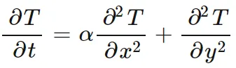
Discretizing the above eqaution by the top down approach as discussed in Steady state,
We end up in ,

The final equation breaks down to,

In addition to the above equation , it must staisfy the CFL criteria which is that
CFL No <= 0.5 to achieve steady state..
Hence the vaue of k1 and k2 should be within 0.5..
PROGRAM CODE FOR TRANSIENT STATE - EXPLICIT FUNCTION
We dont use any point iterative methods here because we have every quantity as the known component..
clear all
close all
clc
L = 1 ;
nx = 10 ;
ny = 10;
x = linspace(0,1,nx);
y = linspace(0,1,ny);
dx = x(2) - x(1) ;
dy = dx ;
t = 300*ones(nx,ny);
% Boundary Conditions
t(2:ny-1,1) = 400;
t(2:ny-1,nx)= 800;
t(1,2:nx-1) = 600;
t(ny,2:nx-1) = 900;
t(1,1) = 500;
t(1,ny) = 700;
t(nx,1) = 650;
t(nx,ny) = 850;
told = t ;
error = 9e9;
tolerance = 1e-4;
dt = 1e-3;
k1= 1.1*(dt/(dx^2));
k2= 1.1*(dt/(dy^2));
iter = 1 ;
while(error>tolerance)
for k=1:1400
for i= 2:nx-1
for j=2:ny-1
term1= told(i,j)
term2 = told(i-1,j) -(2*(told(i,j))) + told(i+1,j)
term3 = told(i,j-1) -(2*(told(i,j))) + told(i,j+1)
t(i,j) = term1+ (k1*term2)+(k2*term3);
end
end
error = max(max(abs(told - t)));
told = t;
iter = iter +1;
end
end
figure(1)
contour(x,y,t)
clabel(contour(x,y,t))
colorbar
colormap(jet)
set(gca,'ydir','reverse')
xlabel('x axis')
ylabel('y axis')
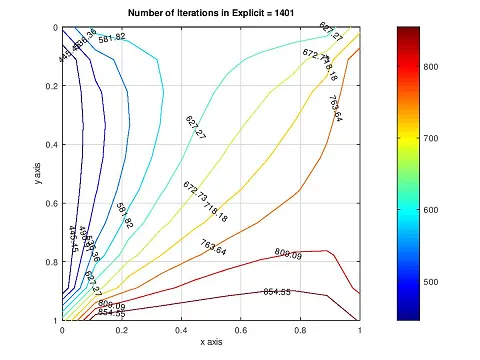
title(sprintf('Number of Iterations in Explicit = %d',iter));
pause(0.03);
PLOT :
UNSTEADY STATE THEORY- IMPLICIT METHOD:
The un steady or Trainsient state is the one which keeps on changing according to time ie; in other words, it is not stable.
The equation of the trainsient involves a term callled diffusivity. Diffusivity is a rate of diffusion, a measure of the rate at which particles or heat or fluids can spread.
Since it is 2D , we take x and y axis ,
Discretizing the above eqaution by the top down approach as discussed in Steady state,
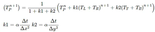
The final equation breaks down to,

PROGRAM CODE FOR TRANSIENT STATE - IMPLICIT - JACOBI METHOD
clear all
close all
clc
L = 1 ;
nx = 10 ;
ny = 10;
x = linspace(0,1,nx)
y = linspace(0,1,ny)
dx = x(2) - x(1) ;
dy = dx ;
t = 300*ones(nx,ny);
% Boundary Conditions
t(2:ny-1,1) = 400;
t(2:ny-1,nx)= 800;
t(1,2:nx-1) = 600;
t(ny,2:nx-1) = 900;
t(1,1) = 500
t(1,ny) = 700
t(nx,1) = 650
t(nx,ny) = 850
t_initial=t;
told = t ;
tolerance = 1e-4;
dt = 1e-3;
k1= 1.1*(dt/(dx^2))
k2= 1.1*(dt/(dy^2))
jacobi_iteration = 1 ;
for k=1:1400
error = 9e9;
while(error>tolerance)
for i= 2:nx-1
for j=2:ny-1
t1 = 1/( 1+(2*k1) +(2*k2));
t2 = k1 *t1;
t3 = k2 * t1;
h= told(i-1,j) + told(i+1,j);
v = told(i,j-1) + told(i,j+1);
t(i,j) = (t_initial(i,j) * t1) + (h*t2) + (v*t3);
end
end
error = max(max(abs(told - t)));
told = t;
jacobi_iteration = jacobi_iteration +1 ;
end
t_initial = t;
end
figure(1)
contour(x,y,t)
clabel(contour(x,y,t))
colorbar
colormap(jet)
set(gca,'ydir','reverse')
xlabel('x axis')
ylabel('y axis')
title(sprintf('Number of Jacobi Iterations = %d',jacobi_iteration));
pause(0.03);
PLOT :
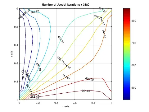
PROGRAM CODE FOR TRANSIENT STATE - IMPLICIT - GAUSS SEIDEL METHOD
clear all
close all
clc
L = 1 ;
nx = 10 ;
ny = 10;
x = linspace(0,1,nx);
y = linspace(0,1,ny);
dx = x(2) - x(1) ;
dy = dx ;
t = 300*ones(nx,ny);
% Boundary Conditions
t(2:ny-1,1) = 400;
t(2:ny-1,nx)= 800;
t(1,2:nx-1) = 600;
t(ny,2:nx-1) = 900;
t(1,1) = 500;
t(1,ny) = 700;
t(nx,1) = 650;
t(nx,ny) = 850;
told = t ;
t_initial=t;
tolerance = 1e-4;
dt = 1e-3;
k1= 1.1*(dt/(dx^2));
k2= 1.1*(dt/(dy^2));
GS_iteration = 1 ;
t1 = 1/( 1+(2*k1) +(2*k2));
t2 = k1 *t1;
t3 = k2 * t1;
for k=1:1400
error = 9e9;
while(error>tolerance)
for i= 2:nx-1
for j=2:ny-1
h= t(i-1,j) + told(i+1,j);
v = t(i,j-1) + told(i,j+1);
t(i,j) = (t_initial(i,j) * t1) + (h*t2) + (v*t3);
end
end
error = max(max(abs(told - t)));
told = t;
GS_iteration = GS_iteration +1 ;
end
t_initial = t;
end
figure(1)
contour(x,y,t)
clabel(contour(x,y,t))
colorbar
colormap(jet)
set(gca,'ydir','reverse')
xlabel('x axis')
ylabel('y axis')
title(sprintf('Number of GS Iterations in Implicit Function = %d',GS_iteration));
pause(0.03);
PLOT :
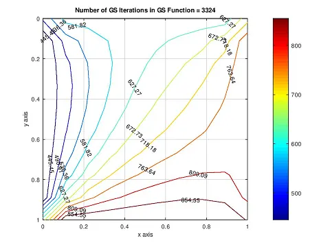
PROGRAM CODE FOR TRANSIENT STATE - IMPLICIT - SUCESSIVE OVER RELAXATION METHOD
clear all
close all
clc
L = 1 ;
nx = 10 ;
ny = 10;
x = linspace(0,1,nx);
y = linspace(0,1,ny);
dx = x(2) - x(1) ;
dy = dx ;
t = 300*ones(nx,ny);
% Boundary Conditions
t(2:ny-1,1) = 400;
t(2:ny-1,nx)= 800;
t(1,2:nx-1) = 600;
t(ny,2:nx-1) = 900;
t(1,1) = 500;
t(1,ny) = 700;
t(nx,1) = 650;
t(nx,ny) = 850;
omega = 1.1 ;
told = t ;
t_initial=t;
t_sor = t;
tolerance = 1e-4;
dt = 1e-3;
k1= 1.1*(dt/(dx^2));
k2= 1.1*(dt/(dy^2));
SOR_iteration = 0 ;
t1 = 1/( 1+(2*k1) +(2*k2))
t2 = k1 *t1
t3 = k2 * t1
for k=1:1400
error = 9e9;
while(error>tolerance)
for i= 2:nx-1
for j=2:ny-1
h= t(i-1,j) + told(i+1,j);
v = t(i,j-1) + told(i,j+1);
t(i,j) = (t_initial(i,j) * t1) + (h*t2) + (v*t3);
t_sor(i,j) = ((1-omega) * told(i,j)) + (omega * t(i,j));
end
end
error = max(max(abs(told - t)));
told = t_sor;
SOR_iteration = SOR_iteration +1 ;
end
t_initial = t_sor;
end
figure(1)
contour(x,y,t)
clabel(contour(x,y,t))
colorbar
colormap(jet)
set(gca,'ydir','reverse')
xlabel('x axis')
ylabel('y axis')
title(sprintf('Number of SOR Iterations in Implicit Function = %d',SOR_iteration));
pause(0.03);
PLOT :
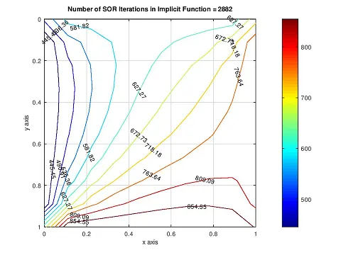
CONCLUSION:
Iterative method is the approximate method which assumes the Values and changing it till the solution reaches a specific point. Unlike the direct methods, which attempts to calculate an exact solution in a finite number of operations, these methods starts with an initial approximation and generate successively improved approximations in an infinite sequence whose limit is the exact solution
From the program codes and results , we come to know that SOR method has a least number of iterations for the error value to be less than the tolerance value in both Steady and Transient State and thereby takes less time naturally and the storage of the SOR solution consumes less memory.When the relaxation factor of SOR is grater than 1 , it becomes an over relaxed solution..