Week 5 - Mid term project - Solving the steady and unsteady 2D heat conduction problem
In this exercise it asked to solve the 2D Heat Equation using different numerical approaches and different type of iterative solvers.
More specifically:
The 2D heat equation is given as:
`(del T)/(del t)+alpha*((del^2 T)/(del x^2)+(del^2 T)/(del y^2)) =0` (1)
And we need to solve the equation considering:
- 2D Heat Equation in Steady-State, using an explicit approach
- Transient 2D Heat equation, using an explicit approach
- Transient 2D Heat equation, using an implicit approach
And within each topic we must use:
- Jacobi method
- Gauss-Seidel method
- Successive over relaxation method (SOR)
The solution to each exercise will be presented by topics. First the derivation and discretization the of parcial differencial equation for the steady-state case will be addressed, Followed by the presentation of the code used to obtainain the solution and the corresponding plots. The same resoning will be applied for the results corresponding to the transient Heat equation.
I) Steady-state heat conduction equation
When considering state-state conditions we are assuming that the solution is no longer a function of time. So in the heat equation, Equation 1, the term corresponding to the time derivative of temperature will be 0.
`(del T)/(del t)=0` (2)
As such the temperature equation for steady-state conditions is given as:
`((del^2 T)/(del x^2)+(del^2 T)/(del y^2)) =0` (3)
For the discretization of this Equation we will be using central differences, which is 2nd order accurate:
`((d^2 T)/(dx^2)+(d^2 T)/(dy^2))= (T_(i-1,j) -2T_(i,j)+T_(i+1,j))/(Delta x^2)+ (T_(i,j-1) -2T_(i,j)+T_(i,j+1))/(Delta y^2)` (4)
for simplification of the notation we will be using:
Temperature at the left node:
`T_L=T_(i-1,j) ;` (5)
Temperature at the right node:
`T_R=T_(i+1,j) ;` (6)
Temperature at the top node:
`T_T=T_(i,j+1) ;` (7)
Temperature at the bottom node:
`T_B=T_(i,j-1) ;` (8)
Temperature at the central node:
`T_P=T_(i,j) ;` (9)
Resulting in:
`((d^2 T)/(dx^2)+(d^2 T)/(dy^2))= (T_L -2T_P+T_R)/(Delta x^2)+ (T_B -2T_P+T_T)/(Delta y^2)` (10)
Isolating the `T_P` therms on the left side of the equation we get:
`T_P*(2/(dx^2)+2/(dy^2))=(1/(dx^2))*(T_L+T_R)+(1/(dy^2))*(T_B+T_T)` (11)
Considering:
`k=(2*dx^2+2*dy^2)/(dx^2*dy^2)` (12)
we obtain:
`T_P=(1/(dx^2*k))*(T_L+T_R)+(1/(dy^2*k))*(T_B+T_T)` (13)
The code use to obtain the solution with 3 different iterative methods is given below:
clear
close all
clc

% Solver for the 2D temperature equation in steady-state using an explicit
% approach
% Points in the x and y direction
nx=11;
ny=11;

% creates a linearly spaced vector for x and y with a length of 1m
x=linspace(0,1,nx);
y=linspace(0,1,ny);

dx=(x(2)-x(1));
dy=(y(2)-y(1));

% Creates a 2D Mesh
T=ones(nx,ny);

% Initiating the field to T=500K
T_init=500;
T=T*T_init;

% Assigning boundary conditions
T_Left=400;
T_Right=800;
T_Top=600;
T_Bottom=900;

T(:,1)=T_Left;
T(:,end)=T_Right;
T(1,:)=T_Top;
T(end,:)=T_Bottom;

% Assigning average properties to the corners
T(1,1)=mean([T_Top T_Left]);
T(end,1)=mean([T_Left T_Bottom]);
T(1,end)=mean([T_Top T_Right]);
T(end,end)=mean([T_Right T_Bottom]);

% Creates a Told variable
Told=T;

% Calculation of k
k=(2*dx^2+2*dy^2)/(dx^2*dy^2);

% Solver parameters
% Define a tolerence for the iterative method
tol = 1e-4;

% initiate the error variable (the value must be higher than the tolerence)
error = 1;


prompt = ['Choose a solver: ',...
          '\n 1. Jacobi',...
          '\n 2. Gauss-Seidel', ...
          '\n 3. SoR \n'];
% Variable to select the type of solver
solver_type=(input(prompt));

% Relaxation parameter in case SOR solver is choosen
w=1.2;

switch solver_type

% jacobi method
case 1
    jacobi_iteration=0;
    while (error > tol)

        for i =2:nx-1
            for j=2:ny-1
                T_1=Told(i-1,j)+Told(i+1,j);
                T_2=Told(i,j-1)+Told(i,j+1);
                T(i,j)=(1/(dx^2*k))*T_1+(1/(dy^2*k))*T_2;
            end
        end


        % calculate the error
        error = max(max(abs(Told-T)));

        % update the temperature field
        Told=T;

        % update the iteration counter
        jacobi_iteration=jacobi_iteration+1;

        contourf(x,y,T);
        c = colorbar;
        c.Label.String = 'Temperature [ºK]';
        xlabel ('x [m]')
        ylabel ('y [m]')
        title(sprintf('Jacobi Method, Iteration number =%d, Error= %0.3d', jacobi_iteration,error))
        set(gca,'ydir','reverse')
        pause(0.001)
    end

    % Gauss-Seidel method
case 2
    gs_iteration=0;
    while (error > tol)

        for i =2:nx-1
            for j=2:ny-1
                T_1=T(i-1,j)+Told(i+1,j);
                T_2=T(i,j-1)+Told(i,j+1);
                T(i,j)=(1/(dx^2*k))*T_1+(1/(dy^2*k))*T_2;
            end
        end


        % calculate the error
        error = max(max(abs(Told-T)));

        % update the temperature field
        Told=T;

        % update the iteration counter
        gs_iteration=gs_iteration+1;

        contourf(x,y,T);
        c = colorbar;
        c.Label.String = 'Temperature [ºK]';
        xlabel ('x [m]')
        ylabel ('y [m]')
        title(sprintf('Gauss-Seidel method, Iteration number =%d, Error= %0.3d', gs_iteration,error))
        set(gca,'ydir','reverse')
        pause(0.001)
    end

        % SOR with Gauss-Siedel Method
case 3
    sor_iteration=0;
    while (error > tol)

        for i =2:nx-1
            for j=2:ny-1
                T_1=T(i-1,j)+Told(i+1,j);
                T_2=T(i,j-1)+Told(i,j+1);
                T_gs(i,j)=(1/(dx^2*k))*T_1+(1/(dy^2*k))*T_2;
                T(i,j)=(1-w)*Told(i,j)+w*(T_gs(i,j));
            end
        end


        % calculate the error
        error = max(max(abs(Told-T)));

        % update the temperature field
        Told=T;

        % update the iteration counter
        sor_iteration=sor_iteration+1;

        contourf(x,y,T);
        c = colorbar;
        c.Label.String = 'Temperature [ºK]';
        xlabel ('x [m]')
        ylabel ('y [m]')
        title(sprintf('SOR method, Iteration number =%d, Error= %0.3d', sor_iteration,error))
        set(gca,'ydir','reverse')
        pause(0.001)
    end

end
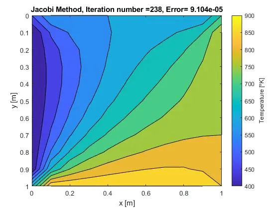
The results with the jacobian method is given in the figure below:
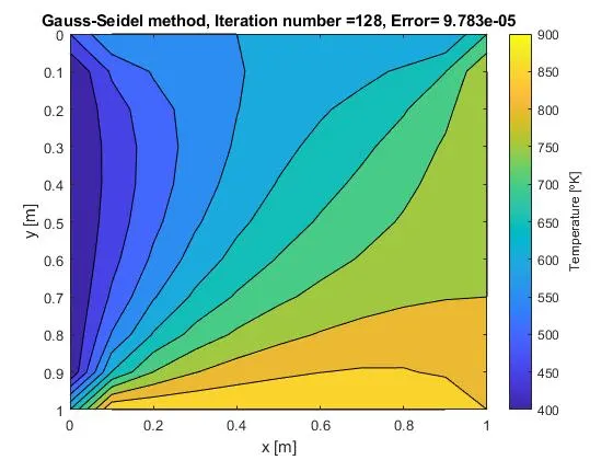
The results with the Gauss-Seidel method is given below:
The results with the SOR method is given below:
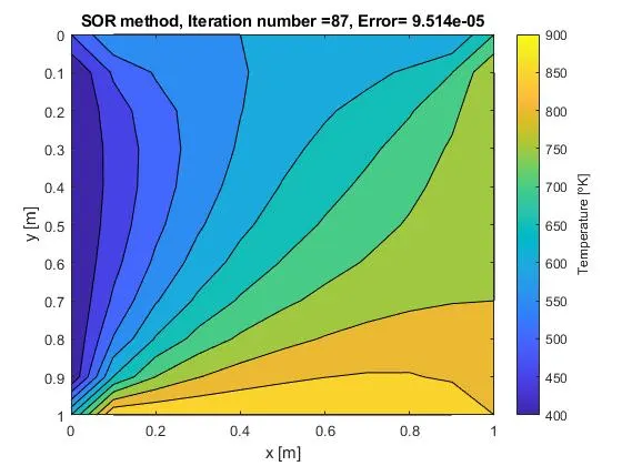
From the results obtained it is possible to observe that the Jacobi method is the slowest to achive convergence (residual<1e-4) with 238 iterations, followed by the Gauss-Seidel method which needed 128 iterations and the fastest methodology is corresponding to the SOR method with 87 iterations.
II) Transient heat conduction equation
a) Using an explicit approach
For this derivation we will start from:
`(del T)/(del t)= alpha*((del^2 T)/(del x^2)+(del^2 T)/(del y^2))` (14)
We will be using forward differences for the time discretization and central differences for the space discretization. Addicionally, the same definitions for the temperature in the left, right, bottom, top and center will be used.
As such equation 14 becomes:
`(T_P^(t+1)-T_P^(t))/(Delta t)=alpha*((T_L^(t)-2T_P^(t)+T_R^(t))/(dx^2)+(T_B^(t)-2T_P^(t)+T_T^(t))/(dy^2))` (15)
Where the superscript t correspondes to the current time, and t+1 to the next time step.
Simplying the equation we get:
`(T_P^(t+1)-T_P^(t))=(alpha*Delta t)/(dx^2)*(T_L^(t)-2T_P^(t)+T_R^(t))+(alpha*Delta t)/(dy^2)(T_B^(t)-2T_P^(t)+T_T^(t))`(16)
Assuming:
`k_1=(alpha*Delta t)/(dx^2)` (17)
`k_2=(alpha*Delta t)/(dy^2)` (18)
We can reorganize equation 16, into:
`(T_P^(t+1)-T_P^(t))=k_1*(T_L^(t)-2T_P^(t)+T_R^(t))+k_2(T_B^(t)-2T_P^(t)+T_T^(t))` (19)
`T_P^(t+1)=T_P^(t)*(1-2k_1-2k_2)+k_1*(T_L^(t)+T_R^(t))+k_2(T_B^(t)+T_T^(t))` (20)
The code used to get the solution in this approach is presented below. The simulation was condidered to reach state-state when the error is less than 1e-4
clear
close all
clc

% Solver for the transient 2D temperature equation using an explicit
% approach
% Points in the x and y direction
nx=11;
ny=11;

% creates a linearly spaced vector for x and y with a length of 1m
x=linspace(0,1,nx);
y=linspace(0,1,ny);

dx=(x(2)-x(1));
dy=(y(2)-y(1));

% Creates a 2D Mesh
T=ones(nx,ny);

% Initiating the field to T=500K
T_init=500;
T=T*T_init;

% Assigning boundary conditions
T_Left=400;
T_Right=800;
T_Top=600;
T_Bottom=900;

T(:,1)=T_Left;
T(:,end)=T_Right;
T(1,:)=T_Top;
T(end,:)=T_Bottom;

% Assigning average properties to the corners
T(1,1)=mean([T_Top T_Left]);
T(end,1)=mean([T_Left T_Bottom]);
T(1,end)=mean([T_Top T_Right]);
T(end,end)=mean([T_Right T_Bottom]);

% Creates a Told variable
Told=T;

% Time related vatiables
dt=1.5e-3;
end_time=2;
nt=end_time/dt;
time=0;

% Define alpha
alpha=1.4;

% Calculation of CFL number for 2D case
k1=((alpha*dt)/(dx^2));
k2=((alpha*dt)/(dy^2));
CFL=k1+k2;


% Solver parameters
% Define a tolerence for the iterative method
tol = 1e-4;

% initiate the error variable (the value must be higher than the tolerence)
error = 1;

prompt = ['Choose a solver: ',...
          '\n 1. Jacobi',...
          '\n 2. Gauss-Seidel', ...
          '\n 3. SoR \n'];
% Variable to select the type of solver
solver_type=(input(prompt));

% Relaxation factor if SOR is used
w=1.2;


switch solver_type

% jacobi method
case 1
    jacobi_iteration=0;
    for k=1:nt
        for i=2:nx-1
            for j=2:ny-1
                T_1=Told(i-1,j)+Told(i+1,j);
                T_2=Told(i,j-1)+Told(i,j+1);
                T(i,j)=Told(i,j)*(1-2*k1-2*k2)+k1*T_1+k2*T_2;
            end
        end


        % calculate the error
        error = max(max(abs(Told-T)));

        % update the temperature field
        Told=T;

        % update the iteration counter
        jacobi_iteration=jacobi_iteration+1;

        % update the time
        time=time+dt;

        % check if error is below the tolerence to consider steady
        % conditions

        contourf(x,y,T);
        c = colorbar;
        c.Label.String = 'Temperature [ºK]';
        xlabel ('x [m]')
        ylabel ('y [m]')
        title(sprintf('Jacobi Method, Iteration number =%d, Error= %0.3d, Time =%3.3f', jacobi_iteration,error,time))
        set(gca,'ydir','reverse')
        pause(0.001)

        % Condition to reach steady-state
        if (tol>error)
            break;
        end
    end

    % Gauss-Seidel method
case 2
    gs_iteration=0;
    for k=1:nt
        for i=2:nx-1
            for j=2:ny-1
                T_1=T(i-1,j)+Told(i+1,j);
                T_2=T(i,j-1)+Told(i,j+1);
                T(i,j)=Told(i,j)*(1-2*k1-2*k2)+k1*T_1+k2*T_2;
            end
        end


        % calculate the error
        error = max(max(abs(Told-T)));

        % update the temperature field
        Told=T;

        % update the iteration counter
        gs_iteration=gs_iteration+1;

        % update the time
        time=time+dt;

        % check if error is below the tolerence to consider steady
        % conditions

        contourf(x,y,T);
        c = colorbar;
        c.Label.String = 'Temperature [ºK]';
        xlabel ('x [m]')
        ylabel ('y [m]')
        title(sprintf('Gauss-Seidel Method, Iteration number =%d, Error= %0.3d, Time =%3.3f', gs_iteration,error,time))
        set(gca,'ydir','reverse')
        pause(0.001)

        % Condition to reach steady-state
        if (tol>error)
            break;
        end
    end

        % SOR method
case 3
    sor_iteration=0;
    for k=1:nt
        for i=2:nx-1
            for j=2:ny-1
                T_1=T(i-1,j)+Told(i+1,j);
                T_2=T(i,j-1)+Told(i,j+1);
                T_gs(i,j)=Told(i,j)*(1-2*k1-2*k2)+k1*T_1+k2*T_2;
                T(i,j)=(1-w)*Told(i,j)+w*(T_gs(i,j));
            end
        end


        % calculate the error
        error = max(max(abs(Told-T)));

        % update the temperature field
        Told=T;

        % update the iteration counter
        sor_iteration=sor_iteration+1;

        % update the time
        time=time+dt;

        % check if error is below the tolerence to consider steady
        % conditions

        contourf(x,y,T);
        c = colorbar;
        c.Label.String = 'Temperature [ºK]';
        xlabel ('x [m]')
        ylabel ('y [m]')
        title(sprintf('SOR Method, Iteration number =%d, Error= %0.3d, Time =%3.3f', sor_iteration,error,time))
        set(gca,'ydir','reverse')
        pause(0.001)

        % Condition to reach steady-state
        if (tol>error)
            break;
        end
    end

end
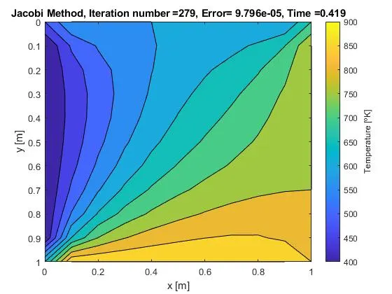
The results for the jacobi method are depicted below:
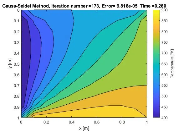
The results for the Gauss-Seidel method are depicted below:
The results for the SOR method are depicted below:
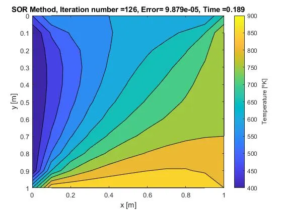
In this approach the time needed to reach steady conditions is the analogous to what was observed in the steady-state problem. The fastest algorithm is the SOR, followed by Gauss-seidel and Jacobi.
b) Using an implicit approach
For the discretization needed in this approach we can recall equation 15 and replace the index t on the right hand side of the equation by t+1, resulting in.
`(T_P^(t+1)-T_P^(t))/(Delta t)=alpha*((T_L^(t+1)-2T_P^(t+1)+T_R^(t+1))/(dx^2)+(T_B^(t+1)-2T_P^(t+1)+T_T^(t+1))/(dy^2))` (21)
Doing a similar simplification to what was performed in the previous topic we get:
`T_P^(t+1)*(1+2*k_1+2*k_2)=T_P^(t)+k_1*(T_L+T_R)+k_2*(T_B+T_T)` (22)
Considering:
`k=(1+2*k_1+2*k_2)` (23)
We obtain:
`T_P^(t+1)=T_P^(t)/k+(k_1/k)*(T_L+T_R)+(k_2/k)*(T_B+T_T)`(24)
The code used to obtain the solution is given below. The solution was considered to reach a steady-state when the difference between the current time step and the previous time step was below 1e-4.
clear
close all
clc

% Solver for the 2D temperature equation in transient using an implicit
% approach
% Points in the x and y direction
nx=11;
ny=11;

% creates a linearly spaced vector for x and y with a length of 1m
x=linspace(0,1,nx);
y=linspace(0,1,ny);

dx=(x(2)-x(1));
dy=(y(2)-y(1));

% Creates a 2D Mesh
T=ones(nx,ny);

% Initiating the field to T=300K
T_init=500;
T=T*T_init;

% Assigning boundary conditions
T_Left=400;
T_Right=800;
T_Top=600;
T_Bottom=900;

T(:,1)=T_Left;
T(:,end)=T_Right;
T(1,:)=T_Top;
T(end,:)=T_Bottom;

% Assigning average properties to the corners
T(1,1)=mean([T_Top T_Left]);
T(end,1)=mean([T_Left T_Bottom]);
T(1,end)=mean([T_Top T_Right]);
T(end,end)=mean([T_Right T_Bottom]);

% Creates a Told variable
Told=T;

% Creates a Tprev variable
Tprev=T;


% Time related vatiables
dt=1.5e-3;
end_time=2;
nt=end_time/dt;
time=0;

% Define alpha
alpha=1.4;

% Calculation of CFL number for 2D case
k1=((alpha*dt)/(dx^2));
k2=((alpha*dt)/(dy^2));
CFL=k1+k2;


% Solver parameters
% Define a tolerence for the iterative method in space and time
tol_space = 1e-4;
tol_time = 1e-4;

% initiate the error variable (the value must be higher than the tolerence)
error = 1;
error_time = 1;
prompt = ['Choose a solver: ',...
          '\n 1. Jacobi',...
          '\n 2. Gauss-Seidel', ...
          '\n 3. SoR \n'];
% Variable to select the type of solver
solver_type=(input(prompt));

% Relaxation factor if SOR is used
w=1.2;


switch solver_type

% jacobi method
case 1
    jacobi_iteration=0;
    while(error_time> tol_time)
        while(error > tol_space)
            for i=2:nx-1
                for j=2:ny-1
                    T_1=Told(i-1,j)+Told(i+1,j);
                    T_2=Told(i,j-1)+Told(i,j+1);
                    k=(1+2*k1+2*k2);
                    T(i,j)=(Tprev(i,j)/k) +(k1/k)*T_1+(k2/k)*T_2;
                end
            end

            % calculate the error
            error = max(max(abs(Told-T)));

            % update the temperature field
            Told=T;

            % update the iteration counter
            jacobi_iteration=jacobi_iteration+1;
        end

        % update the time and
        time=time+dt;

        % Calculates the error between time steps
        error_time=max(max(abs(T-Tprev)));

       % restarts the error variable
        error= 1;

       % update Tprev
        Tprev=T;

        % plots
        contourf(x,y,T);
        c = colorbar;
        c.Label.String = 'Temperature [ºK]';
        xlabel ('x [m]')
        ylabel ('y [m]')
        title(sprintf('Jacobi Method, Iteration number =%d, Error between time steps= %0.3d, Time =%3.3f', jacobi_iteration,error_time,time))
        set(gca,'ydir','reverse')
        pause(0.001)

    end

    % Gauss-seidel method
case 2
    gs_iteration=0;
    while(error_time> tol_time)
        while(error > tol_space)
            for i=2:nx-1
                for j=2:ny-1
                    T_1=T(i-1,j)+Told(i+1,j);
                    T_2=T(i,j-1)+Told(i,j+1);
                    k=(1+2*k1+2*k2);
                    T(i,j)=(Tprev(i,j)/k) +(k1/k)*T_1+(k2/k)*T_2;
                end
            end

            % calculate the error
            error = max(max(abs(Told-T)));

            % update the temperature field
            Told=T;

            % update the iteration counter
            gs_iteration=gs_iteration+1;
        end

        % update the time and
        time=time+dt;

        % Calculates the error between time steps
        error_time=max(max(abs(T-Tprev)));

       % restarts the error variable
        error= 1;

       % update Tprev
        Tprev=T;

        % plots
        contourf(x,y,T);
        c = colorbar;
        c.Label.String = 'Temperature [ºK]';
        xlabel ('x [m]')
        ylabel ('y [m]')
        title(sprintf('Gauss-Seidel Method, Iteration number =%d, Error between time steps= %0.3d, Time =%3.3f', gs_iteration,error_time,time))
        set(gca,'ydir','reverse')
        pause(0.001)

    end

     % SOR method
case 3
    sor_iteration=0;
    while(error_time> tol_time)
        while(error > tol_space)
            for i=2:nx-1
                for j=2:ny-1
                    T_1=T(i-1,j)+Told(i+1,j);
                    T_2=T(i,j-1)+Told(i,j+1);
                    k=(1+2*k1+2*k2);
                    T_gs(i,j)=(Tprev(i,j)/k) +(k1/k)*T_1+(k2/k)*T_2;
                    T(i,j)=(1-w)*Told(i,j)+w*(T_gs(i,j));
                end
            end

            % calculate the error
            error = max(max(abs(Told-T)));

            % update the temperature field
            Told=T;

            % update the iteration counter
            sor_iteration=sor_iteration+1;
        end

        % update the time and
        time=time+dt;

        % Calculates the error between time steps
        error_time=max(max(abs(T-Tprev)));

       % restarts the error variable
        error= 1;

       % update Tprev
        Tprev=T;

        % plots
        contourf(x,y,T);
        c = colorbar;
        c.Label.String = 'Temperature [ºK]';
        xlabel ('x [m]')
        ylabel ('y [m]')
        title(sprintf('SOR Method, Iteration number =%d, Error between time steps= %0.3d, Time =%3.3f', sor_iteration,error_time,time))
        set(gca,'ydir','reverse')
        pause(0.001)

    end


end
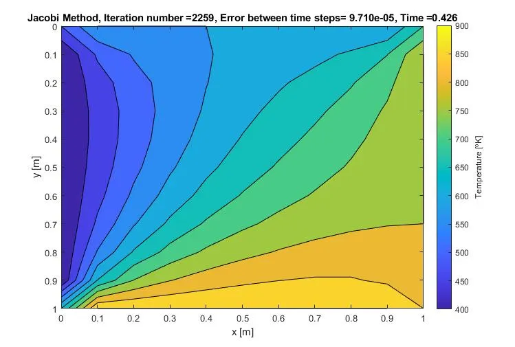
The results for the Jacobi method is:
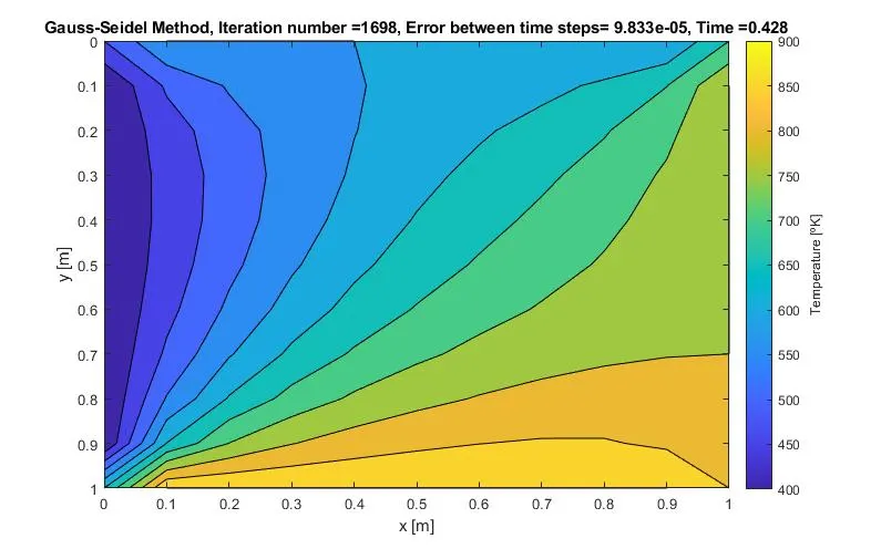
The results for the Gauss-Seidel method:
The results for the SOR method:
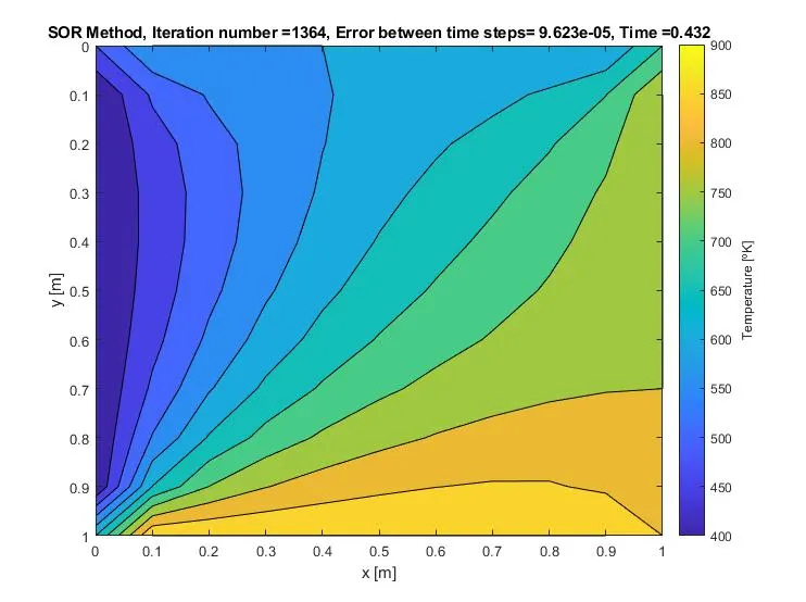
Similar to the previous approaches, the fastest solution is achieved with the SOR method, followed by the Gauss-Siedel and finally the Jacobi method.