Week 5 - Mid term project - Solving the steady and unsteady 2D heat conduction problem
INTRODUCTION
The general heat conduction equation without heat generation in the 2D cartesian coordinate system can be represented as :
`\frac{\partialT}{\partialt} = \alpha(\frac{\partial^2T}{\partialx^2} + \frac{\partial^2T}{\partialy^2})`
where`T` represents the temperature, `t` represents the time, `x` represents the x coordinate and `y` represents the y coordinate.
For the steady-state heat conduction, the equation can be re-written by dropping the time derivative. The steady heat conduction equation can be written as shown below:
`\frac{\partial^2T}{\partialx^2} + \frac{\partial^2T}{\partialy^2} = 0`
In this project, the 2D heat conduction equation, the steady-equation and the transient equation are solved using Numerical iterative techniques such as Jacobi, Gauss-Siedel and Successive Over Relaxation.
The boundary conditions used to solve the 2D heat conduction equation are Dirichlet boundary conditions on all the boundaries. The domain of the mathematical equation is a unit square. The temperature at the left, right, top and bottom walls are specified.
RESULTS AND CODE
First, the steady-state heat conduction equation is solved using Jacobi, Gauss-Siedel and the Successive Over Relaxation methods. The results are plotted and the comparison between the number of iterations and the execution time is made for the different type of solvers.
The discretised form of the steady 2D heat conduction equation is given below:
`\frac{T(i-1,j) -2T(i,j) +T(i+1,j)}{\Deltax^2} + \frac{T(i,j-1) -2T(i,j) +T(i,j+1)}{\Deltay^2}=0`
From the above equation we can write:
`T(i,j) = \frac{\Deltay^2(T(i+1,j)+T(i-1,j)) +\Deltax^2(T(i,j+1)+T(i,j-1))}{2(\Deltax^2 +\Deltay^2)}`
The above equation can be solved iteratively to obtain the temperature distribution inside the unit square for the specified boundary conditions which is
Top Boundary = 600 K, Bottom Boundary = 900 K,Left Boundary = 400 K and Right Boundary = 800 K
The Matlab code is shown below:
clear all;
close all;
clc;
%% Defining the domain and Meshing
Lx = 1;%m
Ly = 1;%m
nx = 30; %No of divisions
ny = nx;
dx = Lx/(nx-1);
dy = Ly/(ny-1);
x = linspace(0,Lx,nx);
y = linspace(0,Ly,ny);

[X,Y] = meshgrid(x,y);

%% Initialisation
T_L = 400;%K
T_R = 800;%K
T_T = 600;%K
T_B = 900;%K

T = 300*ones(nx,ny);

T(2:ny -1,1) = T_L;
T(2:ny -1,nx) = T_R;
T(1,2:nx-1) = T_T;
T(ny,2:nx-1) = T_B;

T(1,1) = (T_L + T_T)/2;
T(nx,ny) = (T_R + T_B)/2;
T(ny,1) = (T_L + T_B)/2;
T(1,nx) = (T_R + T_T)/2;

error = 1e9;
tol = 1e-4;
Told = T;
omega = 1.8;
solver = 3
%% Coefficients

k1 = dx^2/(dx^2 + dy^2);
k2 = dy^2/(dx^2 + dy^2);

%% Jacobi Solver
if solver == 1
jacobi_iter =1;
tic
while (error > tol)
    for i = 2:nx-1
        for j = 2:ny-1

            T(i,j) = 0.5*k1*(Told(i-1,j) + Told(i+1,j)) + 0.5*k2*(Told(i,j-1) + Told(i,j+1));

        end

    end
     error = max(max(abs(Told -T)));
     Told = T;
     jacobi_iter = jacobi_iter+1

end
toc
run_time_jacobi = toc
% Plot Figure for Jacobi iteration
figure(1)
[M,N]=contourf(X,Y,T);
clabel(M,N)
colormap(hot)
colorbar
title_text=sprintf('Jacobi Steady iteration number =%d ,Total Time F=%fs',jacobi_iter,run_time_jacobi);
title(title_text)
xlabel('X-axis')
ylabel('Y-axis')
fprintf('No of Iteration in jacobi=%d\n',jacobi_iter);
end

%% Solver Gauss_Siedel
if solver == 2
gauss_siedel_iter =1;
tic
while (error > tol)
    for i = 2:nx-1
        for j = 2:ny-1

            T(i,j) = 0.5*k1*(T(i-1,j) + Told(i+1,j)) + 0.5*k2*(T(i,j-1) + Told(i,j+1));

        end

    end
     error = max(max(abs(Told -T)));
     Told = T;
     gauss_siedel_iter = gauss_siedel_iter+1

end
toc
run_time_gauss_siedel = toc
% Plot Figure for Gauss Siedel iteration
figure(2)
[M,N]=contourf(X,Y,T);
clabel(M,N)
colormap(hot)
colorbar
title_text=sprintf('Gauss-Siedel Steady iteration number =%d ,Total Time F=%fs',gauss_siedel_iter,run_time_gauss_siedel);
title(title_text)
xlabel('X-axis')
ylabel('Y-axis')
fprintf('No of Iteration in gauss s=%d\n',gauss_siedel_iter);
end
%% SOR Solver
if solver == 3
sor_iter =1;
tic
while (error > tol)
    for i = 2:nx-1
        for j = 2:ny-1

            T(i,j) = ((1 -omega)*Told(i,j)) + omega*(0.5*k1*(T(i-1,j) + Told(i+1,j)) + 0.5*k2*(T(i,j-1) + Told(i,j+1)));

        end

    end
     error = max(max(abs(Told -T)));
     Told = T;
     sor_iter = sor_iter+1

end
toc
run_time_sor = toc
% Plot Figure for Jacobi iteration
figure(3)
[M,N]=contourf(X,Y,T);
clabel(M,N)
colormap(hot)
colorbar
title_text=sprintf('SOR Steady iteration number =%d ,Total Time F=%fs',sor_iter,run_time_sor);
title(title_text)
xlabel('X-axis')
ylabel('Y-axis')
fprintf('No of Iteration in SOR=%d\n',sor_iter);
end
The above code defines the three different solvers for solving the 2D steady-state heat conduction equation. The step-wise explanation of the code is given below:
%% Defining the domain and Meshing
Lx = 1;%m
Ly = 1;%m
nx = 30; %No of divisions
ny = nx;
dx = Lx/(nx-1);
dy = Ly/(ny-1);
x = linspace(0,Lx,nx);
y = linspace(0,Ly,ny);

[X,Y] = meshgrid(x,y);
In the above snippet of code the domain is defined and mesh is created. The domain is a unit square. The length and breadth of the square is defined as Lx and Ly. The domain is equally divided using the linspace() function and the coordinates are generated using the meshgrid() function.
%% Initialisation
T_L = 400;%K
T_R = 800;%K
T_T = 600;%K
T_B = 900;%K

T = 300*ones(nx,ny);

T(2:ny -1,1) = T_L;
T(2:ny -1,nx) = T_R;
T(1,2:nx-1) = T_T;
T(ny,2:nx-1) = T_B;

T(1,1) = (T_L + T_T)/2;
T(nx,ny) = (T_R + T_B)/2;
T(ny,1) = (T_L + T_B)/2;
T(1,nx) = (T_R + T_T)/2;

error = 1e9;
tol = 1e-4;
Told = T;
omega = 1.8;
solver = 1
%% Coefficients

k1 = dx^2/(dx^2 + dy^2);
k2 = dy^2/(dx^2 + dy^2);
The boundary values are initialised as specified in the challenge. The corner points are assigned the values of the average of adjacent nodes. The inner points are assigned a value of 300 K.
The error value and the tolerance values are assigned to variables error and tol. The relaxation factor omega is defined. A variable solver is defined which can be used to select the solvers needed. By changing the value of the solver variable between 1 and 3 we can select Jacobi, Gauss-Siedel or the SOR solver.
%% Jacobi Solver
if solver == 1
jacobi_iter =1;
tic
while (error > tol)
    for i = 2:nx-1
        for j = 2:ny-1

            T(i,j) = 0.5*k1*(Told(i-1,j) + Told(i+1,j)) + 0.5*k2*(Told(i,j-1) + Told(i,j+1));

        end

    end
     error = max(max(abs(Told -T)));
     Told = T;
     jacobi_iter = jacobi_iter+1

end
toc
run_time_jacobi = toc
% Plot Figure for Jacobi iteration
figure(1)
[M,N]=contourf(X,Y,T);
clabel(M,N)
colormap(hot)
colorbar
title_text=sprintf('Jacobi Steady iteration number =%d ,Total Time F=%fs',jacobi_iter,run_time_jacobi);
title(title_text)
xlabel('X-axis')
ylabel('Y-axis')
fprintf('No of Iteration in jacobi=%d\n',jacobi_iter);
end
When the solver variable is assigned the value 1, the above snippet of code gets executed. The solver solves the equation using the Jacobi iteration technique which is a comparatively slow method to converge.
The solution of the equation is presented in a plot as shown below:
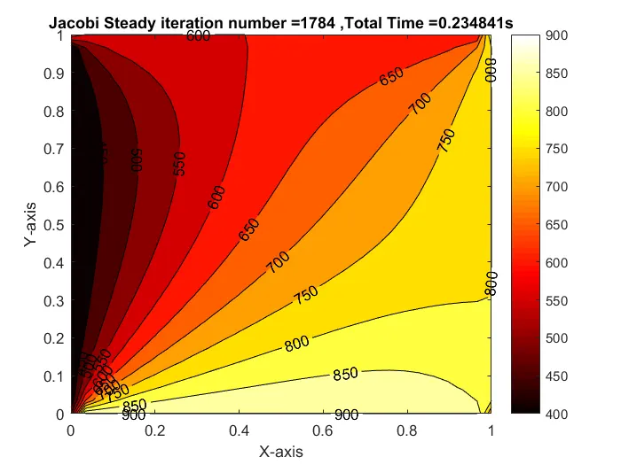
The solution converged at 1784 iterations and it took 0.23 s for generating a converged solution.
The Gauss-Siedeliterative solver is shown below:
%% Solver Gauss_Siedel
if solver == 2
gauss_siedel_iter =1;
tic
while (error > tol)
    for i = 2:nx-1
        for j = 2:ny-1

            T(i,j) = 0.5*k1*(T(i-1,j) + Told(i+1,j)) + 0.5*k2*(T(i,j-1) + Told(i,j+1));

        end

    end
     error = max(max(abs(Told -T)));
     Told = T;
     gauss_siedel_iter = gauss_siedel_iter+1

end
toc
run_time_gauss_siedel = toc
% Plot Figure for Gauss Siedel iteration
figure(2)
[M,N]=contourf(X,Y,T);
clabel(M,N)
colormap(hot)
colorbar
title_text=sprintf('Gauss-Siedel Steady iteration number =%d ,Total Time =%fs',gauss_siedel_iter,run_time_gauss_siedel);
title(title_text)
xlabel('X-axis')
ylabel('Y-axis')
fprintf('No of Iteration in gauss s=%d\n',gauss_siedel_iter);
end
When the value of solver is assigned to be 2 the above snippet of code is executed. The Gauss-Siedel solver converges faster than the Jacobi solver since the values of variables calculated in the current iteration of the previous nodes are used. The plot of the solution is shown below:
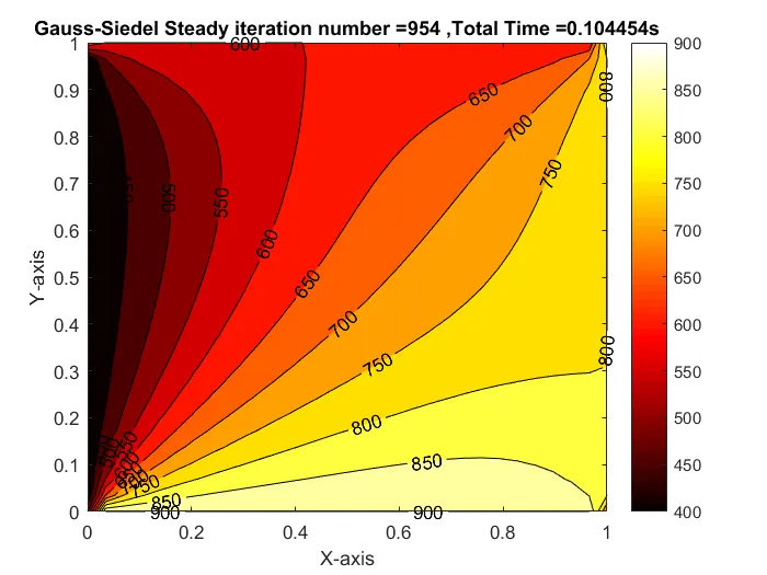
The solution was converged at 954 iterations and the total time taken is 0.10 s.
%% SOR Solver
if solver == 3
sor_iter =1;
tic
while (error > tol)
    for i = 2:nx-1
        for j = 2:ny-1

            T(i,j) = ((1 -omega)*Told(i,j)) + omega*(0.5*k1*(T(i-1,j) + Told(i+1,j)) + 0.5*k2*(T(i,j-1) + Told(i,j+1)));

        end

    end
     error = max(max(abs(Told -T)));
     Told = T;
     sor_iter = sor_iter+1

end
toc
run_time_sor = toc
% Plot Figure for Jacobi iteration
figure(3)
[M,N]=contourf(X,Y,T);
clabel(M,N)
colormap(hot)
colorbar
title_text=sprintf('SOR Steady iteration number =%d ,Total Time F=%fs',sor_iter,run_time_sor);
title(title_text)
xlabel('X-axis')
ylabel('Y-axis')
fprintf('No of Iteration in SOR=%d\n',sor_iter);
end
The above snippet of code gets executed when the solver is assigned a value of 3. The solution easily converges since the variable omega is used to overshoot the values in the next iteration and forces towards convergence faster. The solution is shown in the figure below:
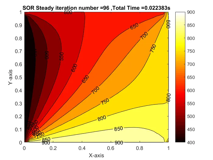
The solution converges at 96 iterations and the solution converges at 0.022 s.
The transient form of 2D heat conduction equation can be discretised and solved in two ways, the explicit and the implicit schemes.
The explicit scheme can be easily coded but it is inherently unstable but the implicit scheme, even though its hard to code is inherently stable.
The discretised form of the 2D transient heat conduction equation is shown below:
`\frac{T^(n+1)(i,j)-T^(n)(i,j)}{\Deltat} = \alpha [\frac{T(i-1,j) -2T(i,j) +T(i+1,j)}{\Deltax^2} + \frac{T(i,j-1) -2T(i,j) +T(i,j+1)}{\Deltay^2}]`
So we can write the temperature in the next step
`T^(n+1)(i,j) = T^(n)(i,j) + \frac{\alpha\Deltat}{\Deltax^2}(T^(n)(i-1,j)-2T^(n)(i,j)+T^(n)(i+1,j)) + \frac{\alpha\Deltat}{\Deltay^2}(T^(n)(i,j-1)-2T^(n)(i,j)+T^(n)(i,j+1))`
The above scheme can be executed without any iterative solvers. The only thing that one should consider is that the sum of the CFL number in the x and y directions must be less than or equal to 0.5.
`Co_x +Co_y<= 0.5`
where, `Co_x = \frac{\alpha\Deltat}{\Deltax^2}` and `Co_y = \frac{\alpha\Deltat}{\Deltay^2}`.
The explicit scheme is implemented using Matlab and is shown below:
%% Defining the domain and Meshing
Lx = 1;%m
Ly = 1;%m
nx = 30; %No of divisions
ny = nx;
dx = Lx/(nx-1);
dy = Ly/(ny-1);
x = linspace(0,Lx,nx);
y = linspace(0,Ly,ny);

[X,Y] = meshgrid(x,y);

%% Initialisation
T_L = 400;%K
T_R = 800;%K
T_T = 600;%K
T_B = 900;%K

T = 300*ones(nx,ny);

T(2:ny -1,1) = T_L;
T(2:ny -1,nx) = T_R;
T(1,2:nx-1) = T_B;
T(ny,2:nx-1) = T_T;

T(1,1) = (T_L + T_T)/2;
T(nx,ny) = (T_R + T_B)/2;
T(ny,1) = (T_L + T_B)/2;
T(1,nx) = (T_R + T_T)/2;

tol = 1e-4;

alpha = 1.4 % Thermal diffusivity for  some arbritary material
solver = 1;
t=50;
dt = 0.0001;
n =t/dt
kx = (alpha*dt)/dx^2  % CFL_x
ky = (alpha*dt)/dy^2  %CFL_y


Told = T;
T_prev = Told;
%% Explicit Method
if solver == 1

iteration = 0

for l = 1:n;

    for i=2:nx-1;
        for j=2:ny-1;
            H = kx*(Told(i-1,j)+Told(i+1,j)- (2*Told(i,j)))
            V = ky*(Told(i,j-1)+Told(i,j+1)- (2*Told(i,j)))
            T(i,j) = Told(i,j)+ H +V

        end
        Told = T;

    end
    iteration =iteration+1

    figure(1)
[M,N]=contourf(X,Y,T);
clabel(M,N)
colormap(hot)
colorbar
title_text=sprintf('Transient Explicit,time step=%d ',iteration);
title(title_text)
xlabel('X-axis')
ylabel('Y-axis')
pause(0.05)
 if( abs(T-T_prev) < 1e-4)
     break
 end

  T_prev = T;

end

end
The time step is set as dt = 0.0001, the thermal diffusivity is taken as alpha = 1.8. The CFL number in the x and y direction is set such that the stability criteria is satisfied. The simulation is set to run for 600 iterations using the initial time loop. There is no need for a convergence loop, the two other loops are spatial loops where the temperature at each spatial points are calculated using the known values of temperatures. The process is continued until the steady-state solution is achieved.
The solution of the explicit solution is shown below:
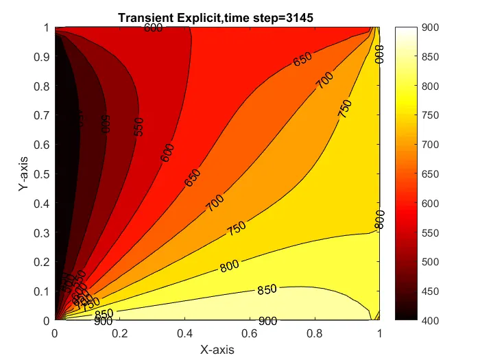
This is the solution to the explicit method for 3145 time steps since each time step is very small the solution converges very slowly.
The implicit scheme for the 2D transient heat conduction equation is shown below:
`T^{n+1}(i,j)=\frac{1}{1+2k_x +2k_y}(T^n(i,j)) + \frac{k_x}{1+2k_x +2k_y}(T^{n+1}(i-1,j)+T^{n+1}(i+1,j)) +\frac{k_y}{1+2k_x +2k_y}(T^{n+1}(i,j-1)+T^{n+1}(i,j+1))`
Since unknown terms are present in the RHS of the equation an iterative solver is required to solve the explicit heat conduction equation. The main advantage of the Implicit method is that the solution is stable irrespective of the CFL number and therefore large time steps can be used and the solution will converge much faster.
The code is written in Matlab to implement the implicit scheme is shown below:
clear all;
close all;
clc;
%% Defining the domain and Meshing
Lx = 1;%m
Ly = 1;%m
nx = 30; %No of divisions
ny = nx;
dx = Lx/(nx-1);
dy = Ly/(ny-1);
x = linspace(0,Lx,nx);
y = linspace(0,Ly,ny);

[X,Y] = meshgrid(x,y);

%% Initialisation
T_L = 400;%K
T_R = 800;%K
T_T = 600;%K
T_B = 900;%K

T = 300*ones(nx,ny);

T(2:ny -1,1) = T_L;
T(2:ny -1,nx) = T_R;
T(1,2:nx-1) = T_B;
T(ny,2:nx-1) = T_T;

T(1,1) = (T_L + T_T)/2;
T(nx,ny) = (T_R + T_B)/2;
T(ny,1) = (T_L + T_B)/2;
T(1,nx) = (T_R + T_T)/2;

tol = 1e-4;

omega = 1.8; % over relaxation factor
alpha = 1.4 % Thermal diffusivity for  some arbritary material
solver = 3;
t=40;
dt = 0.01;
n =t/dt
kx = (alpha*dt)/dx^2  % CFL_x
ky = (alpha*dt)/dy^2  %CFL_y

term1 = (1 + (2*kx) + (2*ky))^-1
term2 = kx*term1
term3 = ky*term1

Told = T;
T_prev = Told;


%% Implicit Jacobi
tic
if solver == 1;
   jacobi_iter = 1;
    jacobi_total_timestep = 1;
    for k = 1:n
        error =100;
        while(error>tol)
            for j = 2:nx-1
                for i = 2:ny-1
                    H = ((Told(i,j+1)) + (Told(i,j-1)));
                    V = ((Told(i+1,j)) + (Told(i-1,j)));
                    T(i,j) = T_prev(i,j)*term1 + H*term2 + V*term3;
                end
            end
            error = max(max(abs(Told-T)));
            Told =T;
            jacobi_iter = jacobi_iter +1;
        end
        [M,N]= contourf(x,y,T)
        clabel(M,N)
        colormap(hot)
        colorbar;
        xlabel('x')
        ylabel('y')
        title_text1 =sprintf('Implicit Jacobi Total Iterations = %d',jacobi_iter);
        title_text2 =sprintf('Total Timesteps = %d',jacobi_total_timestep);
        title({title_text1,title_text2});
        jacobi_total_timestep = jacobi_total_timestep +1;
        pause(0.01)

        if(abs(T-T_prev) < 1e-4)
            break
        end

        T_prev=T;
    end
end
toc
time1 = toc


%% Implicit Gauss-Siedel
tic
if solver == 2
   gs_iter = 1;
    gs_total_timestep = 1;
    for k = 1:n
        error =100;
        while(error>tol)
            for j = 2:nx-1
                for i = 2:ny-1
                    H = ((Told(i,j+1)) + (T(i,j-1)));
                    V = ((Told(i+1,j)) + (T(i-1,j)));
                    T(i,j) = T_prev(i,j)*term1 + H*term2 + V*term3;
                end
            end
            error = max(max(abs(Told-T)));
            Told =T;
            gs_iter = gs_iter +1;
        end
        [M,N]= contourf(x,y,T)
        clabel(M,N)
        colormap(hot)
        colorbar;
        xlabel('x')
        ylabel('y')
        title_text1 =sprintf('Implicit Gauss Siedel Total Iterations = %d',gs_iter);
        title_text2 =sprintf('Total Timesteps = %d',gs_total_timestep);
        title({title_text1,title_text2});
        gs_total_timestep = gs_total_timestep +1;
        pause(0.05)

        if(abs(T-T_prev) < 1e-4)
            break
        end

        T_prev=T;
    end
end
toc
time2 = toc


%% Implicit SOR
tic
if solver == 3
   sor_iter = 1;
    sor_total_timestep = 1;
    for k = 1:n

        error =100;
        while(error>tol)
            for j = 2:nx-1
                for i = 2:ny-1
                    H = ((Told(i,j+1)) + (T(i,j-1)));
                    V = ((Told(i+1,j)) + (T(i-1,j)));
                    T(i,j) = ((1-omega)*Told(i,j)) +(omega*(T_prev(i,j)*term1 + H*term2 + V*term3));
                end
            end
            error = max(max(abs(Told-T)));
            Told =T;
            sor_iter = sor_iter +1;
        end

        [M,N]= contourf(x,y,T);
        clabel(M,N)
        colormap(hot)
        colorbar;
        xlabel('x')
        ylabel('y')
        title_text1 =sprintf('Implicit SOR Total Iterations = %d',sor_iter);
        title_text2 =sprintf('Total Timesteps = %d',sor_total_timestep);
        title({title_text1,title_text2});
        sor_total_timestep = sor_total_timestep +1;
        pause(0.05)
         if(abs(T-T_prev) < 1e-4)
            break
        end
        T_prev=T;
    end
end
toc
time3 = toc
Since the Implicit method is inherently stable the code will not blow up even for high values of the time step. The stepwise explanation of the above code is given below:
clear all;
close all;
clc;
%% Defining the domain and Meshing
Lx = 1;%m
Ly = 1;%m
nx = 30; %No of divisions
ny = nx;
dx = Lx/(nx-1);
dy = Ly/(ny-1);
x = linspace(0,Lx,nx);
y = linspace(0,Ly,ny);

[X,Y] = meshgrid(x,y);

%% Initialisation
T_L = 400;%K
T_R = 800;%K
T_T = 600;%K
T_B = 900;%K

T = 300*ones(nx,ny);

T(2:ny -1,1) = T_L;
T(2:ny -1,nx) = T_R;
T(1,2:nx-1) = T_B;
T(ny,2:nx-1) = T_T;

T(1,1) = (T_L + T_T)/2;
T(nx,ny) = (T_R + T_B)/2;
T(ny,1) = (T_L + T_B)/2;
T(1,nx) = (T_R + T_T)/2;
As explained in the previous cases the above snippet of code meshes the domain and initialise the boundary conditions.
tol = 1e-4;

omega = 1.8; % over relaxation factor
alpha = 1.4 % Thermal diffusivity for  some arbritary material
solver = 3;
t=40;
dt = 0.01;
n =t/dt
kx = (alpha*dt)/dx^2  % CFL_x
ky = (alpha*dt)/dy^2  %CFL_y

term1 = (1 + (2*kx) + (2*ky))^-1
term2 = kx*term1
term3 = ky*term1

Told = T;
T_prev = Told;
In the above snippet of code, the tolerance value is defined as tol, the over-relaxation factor omega is set as 1.8. The Courant number in the x and y direction is defined as kx and ky. The time step value is chosen as dt=0.01 since the implicit scheme is inherently stable irrespective of the Courant number. The solver variable is used to select the solver type which is Jacobi, Gauss-Siedel or SOR solver.
%% Implicit Jacobi
tic
if solver == 1;
   jacobi_iter = 1;
    jacobi_total_timestep = 1;
    for k = 1:n
        error =100;
        while(error>tol)
            for j = 2:nx-1
                for i = 2:ny-1
                    H = ((Told(i,j+1)) + (Told(i,j-1)));
                    V = ((Told(i+1,j)) + (Told(i-1,j)));
                    T(i,j) = T_prev(i,j)*term1 + H*term2 + V*term3;
                end
            end
            error = max(max(abs(Told-T)));
            Told =T;
            jacobi_iter = jacobi_iter +1;
        end
        [M,N]= contourf(x,y,T)
        clabel(M,N)
        colormap(hot)
        colorbar;
        xlabel('x')
        ylabel('y')
        title_text1 =sprintf('Implicit Jacobi Total Iterations = %d',jacobi_iter);
        title_text2 =sprintf('Total Timesteps = %d',jacobi_total_timestep);
        title({title_text1,title_text2});
        jacobi_total_timestep = jacobi_total_timestep +1;
        pause(0.01)

        if(abs(T-T_prev) < 1e-4)
            break
        end

        T_prev=T;
    end
end
toc
time1 = toc
In the above snippet of code, the Jacobi method is used to implement the Implicit scheme. It can be selected by setting solver =1. Inside the time loop, there is a convergence loop which is to be run for each time step. The error value is set as error = 100, inside the time loop before the convergence loop to renew it after every time step. The convergence loop is used since the unknown values are used in solving the linear equation in each time step. The spatial loop is used to calculate the temperature at all the points in the domain. The loop exits when the difference between two adjacent time step is less than 1e-4.
The output of the above code is given below:
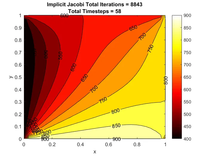
The total number of iterations required for convergence is 8843 and the solution converged in 58 time steps.
The Gauss-Siedel method implemented is shown below:
%% Implicit Gauss-Siedel
tic
if solver == 2
   gs_iter = 1;
    gs_total_timestep = 1;
    for k = 1:n
        error =100;
        while(error>tol)
            for j = 2:nx-1
                for i = 2:ny-1
                    H = ((Told(i,j+1)) + (T(i,j-1)));
                    V = ((Told(i+1,j)) + (T(i-1,j)));
                    T(i,j) = T_prev(i,j)*term1 + H*term2 + V*term3;
                end
            end
            error = max(max(abs(Told-T)));
            Told =T;
            gs_iter = gs_iter +1;
        end
        [M,N]= contourf(x,y,T)
        clabel(M,N)
        colormap(hot)
        colorbar;
        xlabel('x')
        ylabel('y')
        title_text1 =sprintf('Implicit Gauss Siedel Total Iterations = %d',gs_iter);
        title_text2 =sprintf('Total Timesteps = %d',gs_total_timestep);
        title({title_text1,title_text2});
        gs_total_timestep = gs_total_timestep +1;
        pause(0.05)

        if(abs(T-T_prev) < 1e-4)
            break
        end

        T_prev=T;
    end
end
toc
time2 = toc
In the above snippet of code, the Gauss-Siedel algorithm is implemented to check the convergence, the output of the above snippet of code is shown below:
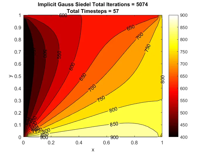
The converged solution was achieved in 5074 iterations and 57 time steps.
The code implementing the successive over-relaxation method is shown below:
%% Implicit SOR
tic
if solver == 3
   sor_iter = 1;
    sor_total_timestep = 1;
    for k = 1:n

        error =100;
        while(error>tol)
            for j = 2:nx-1
                for i = 2:ny-1
                    H = ((Told(i,j+1)) + (T(i,j-1)));
                    V = ((Told(i+1,j)) + (T(i-1,j)));
                    T(i,j) = ((1-omega)*Told(i,j)) +(omega*(T_prev(i,j)*term1 + H*term2 + V*term3));
                end
            end
            error = max(max(abs(Told-T)));
            Told =T;
            sor_iter = sor_iter +1;
        end

        [M,N]= contourf(x,y,T);
        clabel(M,N)
        colormap(hot)
        colorbar;
        xlabel('x')
        ylabel('y')
        title_text1 =sprintf('Implicit SOR Total Iterations = %d',sor_iter);
        title_text2 =sprintf('Total Timesteps = %d',sor_total_timestep);
        title({title_text1,title_text2});
        sor_total_timestep = sor_total_timestep +1;
        pause(0.05)
         if(abs(T-T_prev) < 1e-4)
            break
        end
        T_prev=T;
    end
end
toc
time3 = toc
The SOR algorithm is implemented and the solution converged after 2127 iterations at 57 time steps.
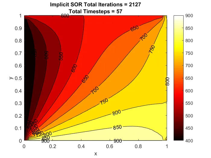
From this, it can be inferred that the SOR method converges the solution faster in the transient Implicit scheme.
CONCLUSION
The code for solving the steady and unsteady heat conduction equation is written in Matlab.
It can be seen that for solving the steady-state equation can be easily solved using different iterative solvers. The Jacobi, Gauss-Siedel and the Successive-Over Relaxation methods are implemented. It is important to note that the SOR solver converges faster with less number of iterations.
The Explicit solution for the transient heat conduction equation requires no iterative solvers since for finding the temperature at the next time step only the known values from the previous time step is only used.
The Implicit solver requires the values of temperature from the current time step for calculation, so an iterative solver is required to calculate the solution. The Jacobi, Gauss-Siedel and the Successive-Over Relaxation methods are implemented. It is important to note that the SOR solver converges faster with less number of iterations.
The time step used in the explicit method is too low so the solution is very slow to converge. Using a larger time step leads to an unstable solution. The implicit method is inherently stable and so we can use larger time steps and the solution can converge much faster than the explicit scheme.