Week 5 - Mid term project - Solving the steady and unsteady 2D heat conduction problem

Aim:

1. Solve the 2D heat conduction equation by using the point iterative techniques that were taught in the class. The Boundary conditions for the problem are as follows;

Top Boundary = 600 K

Bottom Boundary = 900

Left Boundary = 400 K

Right Boundary = 800 K

Method to Implement:

1. Jacobi
2. Gauss-seidel
3. Successive over-relaxation

2. Write code for both implicit and explicit schemes (For the Transient Analysis only)

Formulation:

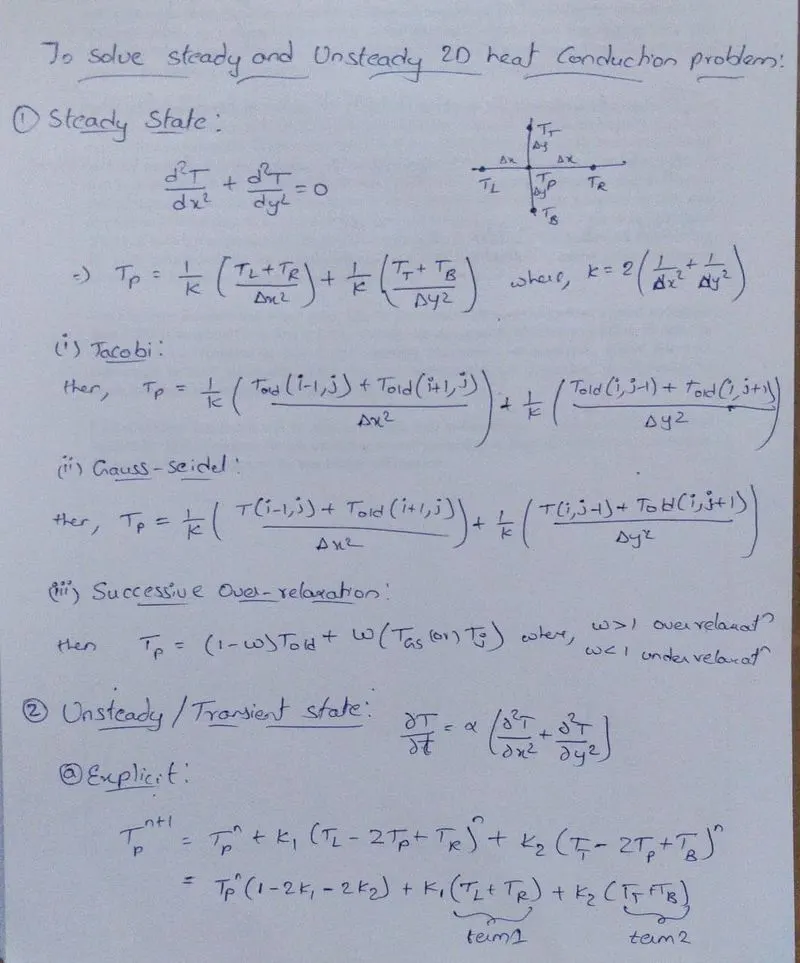
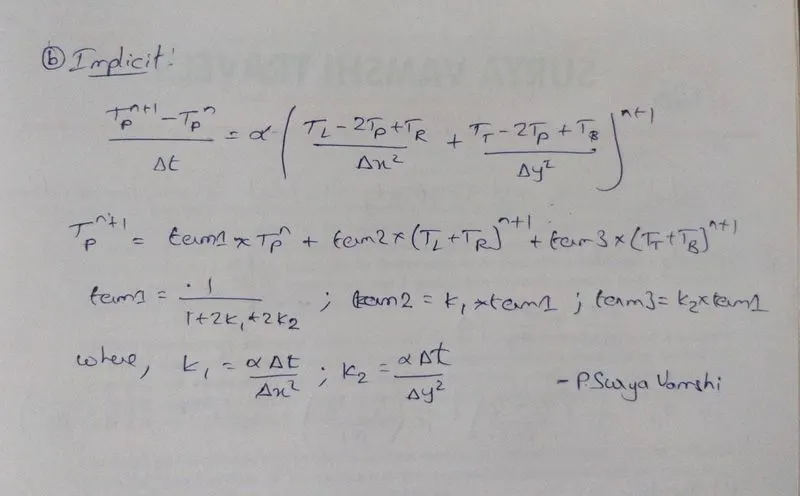
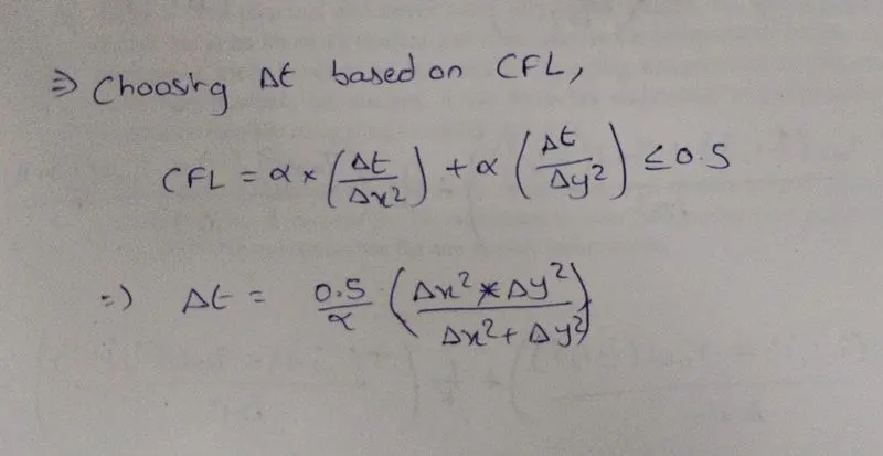
For Transient or Unsteady state, delta-t is calculated using,

MATLAB Program:

I have added comments wherever necessary to make sure everyone can understand.

It follows the following pattern:

1. Main code: Contains the initial inputs and some necessary constants calculation. Then the functions are called accordingly to solve the equation. They will return the number of iteration and I had plotted a separate graph to visualize it.
2. Then the rest of the code is individual functions which take inputs from the main code and solve accordingly.

Main code:

%% To Solve the 2D heat conduction equation by using the point iterative techniques
%% Inputs (Which does not change with type of study)
l = 1;      % Length of given domain
nx = 10;    % Number of Grid Points Along X-axis
ny = nx;    % Number of Grid Points Along Y-axis
x = linspace(0,l,nx);     % Creating grids Along X-axis
y = linspace(0,l,ny);     % Creating grids Along Y-axis
dx = l/(nx-1);    % Distance Between Two Grid Points Along X-axis
dy = l/(ny-1);    % Distance Between Two Grid Points Along Y-axis

tol = 1e-4;    % Tolerance Limit
%% Assigning temperatures 
Temp = 300*ones(nx,ny); % Inital Temperature at every point
% Temperature at boundaries
Temp(:,1) = 400;     % Temperature at Left Boundary
Temp(:,end) = 800;   % Temperature at Right Boundary
Temp(1,:) = 600;     % Temperature at Top Boundary
Temp(end,:) = 900;   % Temperature at Bottom Boundary
% Calculating Average of Temperature at the ends
Temp(1,1) = (600+400)/2;
Temp(1,end) = (600+800)/2;
Temp(end,1) = (900+400)/2;
Temp(end,end) = (900+800)/2;

%% Solving Steady state 2D heat conduction equation using Iterative Methods
% Constant In Steady State Equation
k = 2*(1/(dx^2)+1/(dy^2));
% Solving
Steady_state_jacobi = ss_jacobi(nx, ny, x, y, dx, dy, Temp, tol, k);
Steady_state_gauss_seidel = ss_gauss_seidel(nx, ny, x, y, dx, dy, Temp, tol, k);
Steady_state_SOR = ss_SOR(nx, ny, x, y, dx, dy, Temp, tol, k);

%% Results of Steady State: Plotting
figure(4)
type = categorical({'Jacobi','Gauss-Siedal','SOR with GS'});
data = [Steady_state_jacobi;Steady_state_gauss_seidel;Steady_state_SOR];
bar(type,data);
xlabel('Iterative Methods Used')
ylabel('Number of iteration')
title('Steady State Iterative Methods (For error less than 1e^-4)')

%% Solving Transient or Unsteady state 2D heat conduction equation using Iterative Methods
% Time Inputs
nt = 1400;
alpha = 1.5;   % Thermal diffusivity 
dt = (0.5*(dy^2)*(dx^2))*(alpha*((dx^2)+(dy^2)))^(-1); % According CFL stability criteria
%number of time steps

% Constants In Unsteady State Equation
k1 = alpha*(dt/dx^2);
k2 = alpha*(dt/dy^2);
% Solving
Unsteady_state_explicit = uss_explicit(nx, ny, x, y, Temp, nt, tol, k1, k2);
Unsteady_state_implicit_jacobi = uss_implicit_jacobi(nx, ny, x, y, Temp, nt, tol, k1, k2);
Unsteady_state_implicit_gauss_seidel = uss_implicit_gauss_seidel(nx, ny, x, y, Temp, nt, tol, k1, k2);
Unsteady_state_implicit_SOR = uss_implicit_SOR(nx, ny, x, y, Temp, nt, tol, k1, k2);

%% Results of Transient or Unsteady State: Plotting
figure(9) 
type = categorical({'Explicit','Implicit-Jacobi','Implicit-GS','Implicit-SOR with GS'});
data=[Unsteady_state_explicit;Unsteady_state_implicit_jacobi;Unsteady_state_implicit_gauss_seidel;Unsteady_state_implicit_SOR];
bar(type,data);
xlabel('Iterative Methods Used')
ylabel('Number of iteration')
title('Transient or Unsteady State Iterative Methods (For error less than 1e^-4)')

Function 1: Steady-State Jacobi

function output = ss_jacobi(nx, ny, x, y, dx, dy, Temp, tol, k)
% ss_jacobi means Steady State Jacobi
meshgrid(x,y);% Creating a 2d grid
Temp_old = Temp;% Creating a copy of Temperature
jacobi_iter = 1; % To count the iterations taken
error = 9e9;% Initial error to run first time
tic % To start recording computation Time

while (error > tol)
    for i = 2:nx-1
        for j = 2:ny-1
            term1 = (Temp_old(i-1,j) + Temp_old(i+1,j))/(k*(dx^2));
            term2 = (Temp_old(i,j-1) + Temp_old(i,j+1))/(k*(dy^2));
            Temp(i,j) = term1 + term2;
        end
    end
    error = max(max(abs(Temp_old - Temp))); % Calculating absolute error
    Temp_old = Temp;   % Updating Temperature
    jacobi_iter = jacobi_iter + 1;
end
iter_time = toc;% To stop recording computation Time
%% Ploting
figure(1)
[a, b] = contourf(x, y, Temp);
colormap(jet)
clabel(a, b);
xlabel('X Direction');
ylabel('Y Direction');
set(gca,'YDIR','reverse')
text1 = sprintf('Error = %f', error);
text2 = sprintf('Jacobi Iterations = %d', jacobi_iter);
text3 = sprintf('Jacobi Simulation Time = %f sec', iter_time);
colorbar
title({'Steady State:';text1;text2;text3});
output = jacobi_iter;
end

Function 2: Steady-State Gauss Seidel

function output = ss_gauss_seidel(nx, ny, x, y, dx, dy, Temp, tol, k)
% ss_gauss_seidel means Steady State Gauss Seidel
meshgrid(x,y);% Creating a 2d grid
Temp_old = Temp;% Creating a copy of Temperature
gs_iter = 1;% To count the iterations taken
error = 9e9;% Initial error to run first time
tic % To start recording computation Time

while (error > tol)
    for i = 2:nx-1
        for j = 2:ny-1
            term1 = (Temp(i-1,j) + Temp_old(i+1,j))/(k*(dx^2));
            term2 = (Temp(i,j-1) + Temp_old(i,j+1))/(k*(dy^2));
            Temp(i,j) = term1 + term2;
        end
    end
    error = max(max(abs(Temp_old - Temp)));
    Temp_old = Temp;   % Updating Temperature
    gs_iter = gs_iter + 1;
end
iter_time = toc;% To stop recording computation Time
%% Ploting
figure(2)
[a, b] = contourf(x, y, Temp);
colormap(jet)
clabel(a, b);
xlabel('X Direction');
ylabel('Y Direction');
set(gca,'YDIR','reverse')
text1 = sprintf('Error = %f', error);
text2 = sprintf('Gauss-Seidel Iterations = %d', gs_iter);
text3 = sprintf('Gauss-Seidel Simulation Time = %f sec', iter_time);
colorbar
title({'Steady State:';text1;text2;text3});
output = gs_iter;
end

Function 3: Steady-State Successive Over-Relaxation

function output= ss_SOR(nx, ny, x, y, dx, dy, Temp, tol, k)
% ss_SOR means Steady State Successive Over-Relaxation
meshgrid(x,y);% Creating a 2d grid
omega = 1.1;  % Over Relaxation Factor
Temp_old = Temp;% Creating a copy of Temperature
sor_iter = 1; % To count the iterations taken
error = 9e9;% Initial error to run first time
tic % To start recording computation Time
while (error > tol)
    for i = 2:nx-1
        for j = 2:ny-1
            term1 = (Temp(i-1,j) + Temp_old(i+1,j))/(k*(dx^2));
            term2 = (Temp(i,j-1) + Temp_old(i,j+1))/(k*(dy^2));
            Temp(i,j) = Temp_old(i,j)*(1-omega) + omega*(term1 + term2);
        end
    end
    error = max(max(abs(Temp_old - Temp)));
    Temp_old = Temp;  % Updating Temperature
    sor_iter = sor_iter + 1;
end
iter_time = toc;% To stop recording computation Time
%% Ploting
figure(3)
[a, b] = contourf(x, y, Temp);
colormap(jet)
clabel(a, b);
xlabel('X Direction');
ylabel('Y Direction');
set(gca,'YDIR','reverse')
text1 = sprintf('Error = %f', error);
text2 = sprintf('Successive Over-Relaxation Iterations = %d', sor_iter);
text3 = sprintf('Successive Over-Relaxation Simulation Time = %f sec', iter_time);
colorbar
title({'Steady State:';text1;text2;text3});
output = sor_iter;
end

Function 4: Unsteady State Explicit

function output = uss_explicit(nx, ny, x, y, Temp, nt, tol, k1, k2)
% uss_explicit means Unsteady State Explicit
meshgrid(x,y);% Creating a 2d grid
Temp_old = Temp; % Creating a copy of Temperature
Temp_prev = Temp; % Creating a copy of Temperature for previous iteration
explicit_iter = 1; % To count the iterations taken
error = 9e9;% Initial error to run first time
tic % To start recording computation Time
for  k = 1:nt
    while (error > tol)
        for i = 2:nx-1
            for j = 2:ny-1
                term1 = (Temp_old(i-1,j) + Temp_old(i+1,j));
                term2 = (Temp_old(i,j-1) + Temp_old(i,j+1));
                Temp(i,j) =(Temp_prev(i,j)*(1 - 2*k1 - 2*k2) + (k1*term1) + (k2*term2));
            end
        end
        error = max(max(abs(Temp_old - Temp)));
        Temp_old = Temp;   % Updating Temperature
        Temp_prev = Temp;  % Updating Temperature as previous iteration
        explicit_iter = explicit_iter + 1;
    end
end
iter_time = toc;% To stop recording computation Time
%% Ploting
figure(5)
[a, b] = contourf(x, y, Temp);
colormap(jet)
clabel(a, b);
xlabel('X Direction');
ylabel('Y Direction');
set(gca,'YDIR','reverse')
text1 = sprintf('Error = %f', error);
text2 = sprintf('Explicit Iterations = %d', explicit_iter);
text3 = sprintf('Explicit Simulation Time = %f sec', iter_time);
colorbar
title({'Transient/Unsteady State:';text1;text2;text3});
output = explicit_iter;
end

Function 5: Unsteady State Implicit with Jacobi

function output = uss_implicit_jacobi(nx, ny, x, y, Temp, nt, tol, k1, k2)
% uss_explicit means Unsteady State Implicit with Jacobi
meshgrid(x,y);% Creating a 2d grid
Temp_old = Temp; % Creating a copy of Temperature
Temp_prev = Temp; % Creating a copy of Temperature for previous iteration
jacobi_iter = 1; % To count the iterations taken
error = 9e9;% Initial error to run first time
tic % To start recording computation Time
for  k = 1:nt
    while (error > tol)
        for i = 2:nx-1
            for j = 2:ny-1
                term1 = (Temp_old(i-1,j) + Temp_old(i+1,j));
                term2 = (Temp_old(i,j-1) + Temp_old(i,j+1));
                Temp(i,j) =(Temp_prev(i,j) + (k1*term1) + (k2*term2))/(1 + 2*k1 + 2*k2);
            end
        end
        error = max(max(abs(Temp_old - Temp)));
        Temp_old = Temp;   % Updating Temperature
        Temp_prev = Temp;  % Updating Temperature as previous iteration
        jacobi_iter = jacobi_iter + 1;
    end
end
iter_time = toc;% To stop recording computation Time
%% Ploting
figure(6)
[a, b] = contourf(x, y, Temp);
colormap(jet)
clabel(a, b);
xlabel('X Direction');
ylabel('Y Direction');
set(gca,'YDIR','reverse')
text1 = sprintf('Error = %f', error);
text2 = sprintf('Implicit Jacobi Iterations = %d', jacobi_iter);
text3 = sprintf('Implicit Jacobi Simulation Time = %f sec', iter_time);
colorbar
title({'Transient/Unsteady State:';text1;text2;text3});
output = jacobi_iter;
end

Function 6: Unsteady State Implicit with Gauss-Seidel

function output = uss_implicit_gauss_seidel(nx, ny, x, y, Temp, nt, tol, k1, k2)
% uss_explicit means Unsteady State Implicit with Gauss Seidel
meshgrid(x,y);% Creating a 2d grid
Temp_old = Temp; % Creating a copy of Temperature
Temp_prev = Temp; % Creating a copy of Temperature for previous iteration
gs_iter = 1; % To count the iterations taken
error = 9e9;% Initial error to run first time
tic % To start recording computation Time
for  k = 1:nt
    while (error > tol)
        for i = 2:nx-1
            for j = 2:ny-1
                term1 = (Temp(i-1,j) + Temp_old(i+1,j));
              term2 = (Temp(i,j-1) + Temp_old(i,j+1));
              Temp(i,j) =(Temp_prev(i,j) + (k1*term1) + (k2*term2))/(1 + 2*k1 + 2*k2);
            end
        end
        error = max(max(abs(Temp_old - Temp)));
        Temp_old = Temp;   % Updating Temperature
        Temp_prev = Temp;  % Updating Temperature as previous iteration
        gs_iter = gs_iter + 1;
    end
end
iter_time = toc;% To stop recording computation Time
%% Ploting
figure(7)
[a, b] = contourf(x, y, Temp);
colormap(jet)
clabel(a, b);
xlabel('X Direction');
ylabel('Y Direction');
set(gca,'YDIR','reverse')
text1 = sprintf('Error = %f', error);
text2 = sprintf('Implicit Gauss Seidel Iterations = %d', gs_iter);
text3 = sprintf('Implicit Gauss Seidel Simulation Time = %f sec', iter_time);
colorbar
title({'Transient/Unsteady State:';text1;text2;text3});
output = gs_iter;
end

Function 7: Unsteady State Implicit with Successive Over-Relaxation with Gauss-Seidel

function output = uss_implicit_SOR(nx, ny, x, y, Temp, nt, tol, k1, k2)
% uss_explicit means Unsteady State Implicit with Successive Over-Relaxation
meshgrid(x,y);% Creating a 2d grid
omega = 1.1;    % Over Realaxation factor
Temp_old = Temp; % Creating a copy of Temperature
Temp_prev = Temp; % Creating a copy of Temperature for previous iteration
SOR_iter = 1; % To count the iterations taken
error = 9e9;% Initial error to run first time
tic % To start recording computation Time
for  k = 1:nt
    while (error > tol)
        for i = 2:nx-1
            for j = 2:ny-1
                term1 = (Temp(i-1,j) + Temp_old(i+1,j));
              term2 = (Temp(i,j-1) + Temp_old(i,j+1));
              Temp(i,j) = Temp_old(i,j)*(1-omega) + omega*(Temp_prev(i,j) + (k1*term1) + (k2*term2))/(1 + 2*k1 + 2*k2);
            end
        end
        error = max(max(abs(Temp_old - Temp)));
        Temp_old = Temp;   % Updating Temperature
        Temp_prev = Temp;  % Updating Temperature as previous iteration
        SOR_iter = SOR_iter + 1;
    end
end
iter_time = toc;% To stop recording computation Time
%% Ploting
figure(8)
[a, b] = contourf(x, y, Temp);
colormap(jet)
clabel(a, b);
xlabel('X Direction');
ylabel('Y Direction');
set(gca,'YDIR','reverse')
text1 = sprintf('Error = %f', error);
text2 = sprintf('Implicit Successive Over-Relaxation Iterations = %d', SOR_iter);
text3 = sprintf('Implicit Successive Over-Relaxation Simulation Time = %f sec', iter_time);
colorbar
title({'Transient/Unsteady State:';text1;text2;text3});
output = SOR_iter;
end

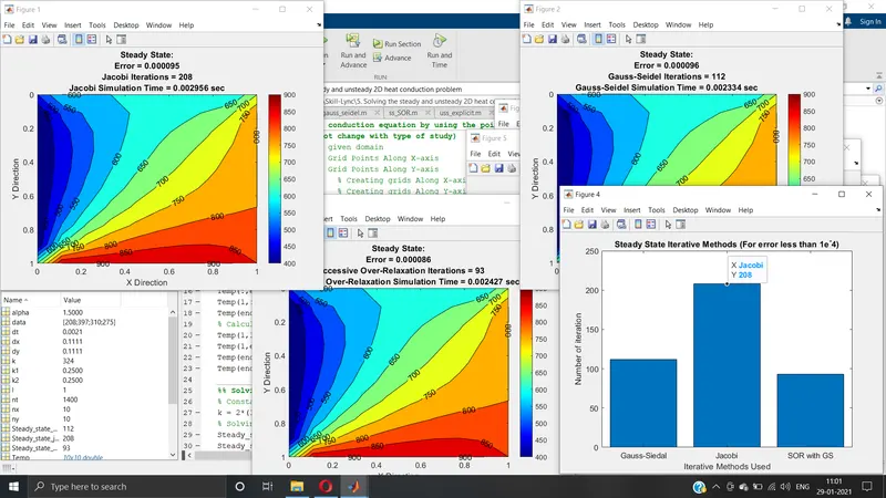
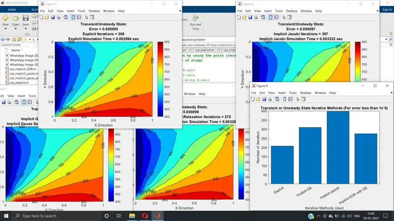
Screenshots:

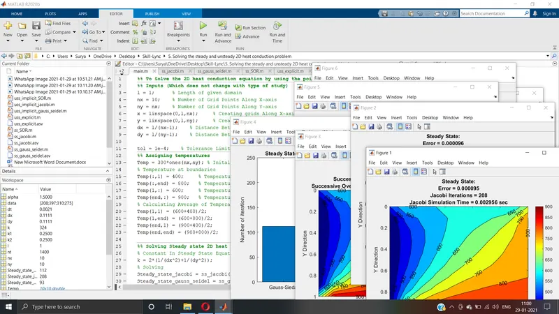
Results:

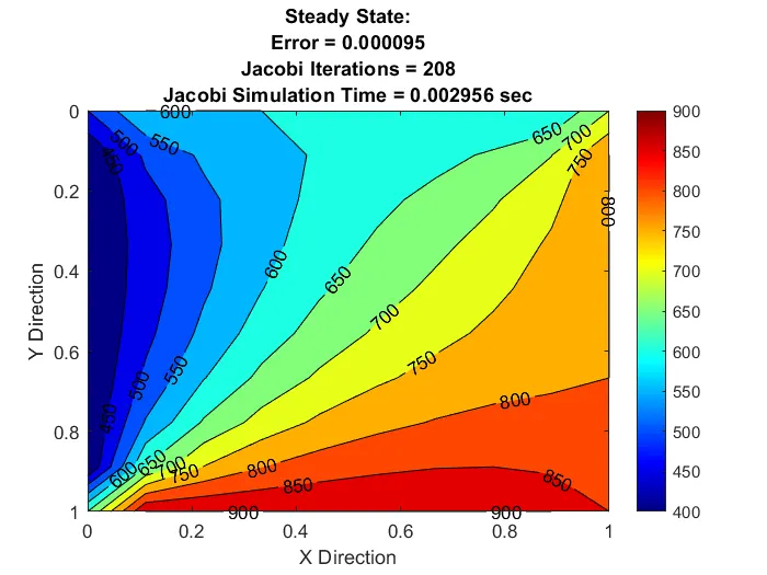
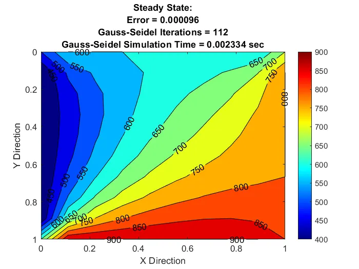
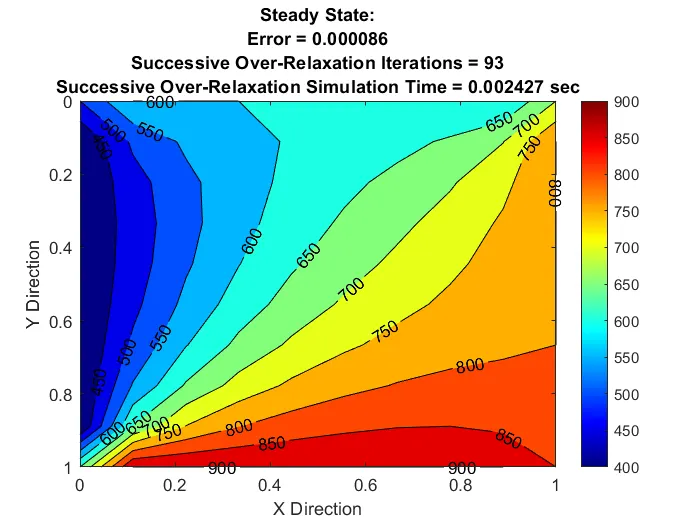
For Steady-state:

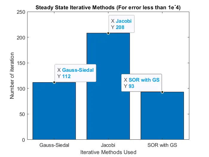
Now, a comparison of steady-state iterative methods.

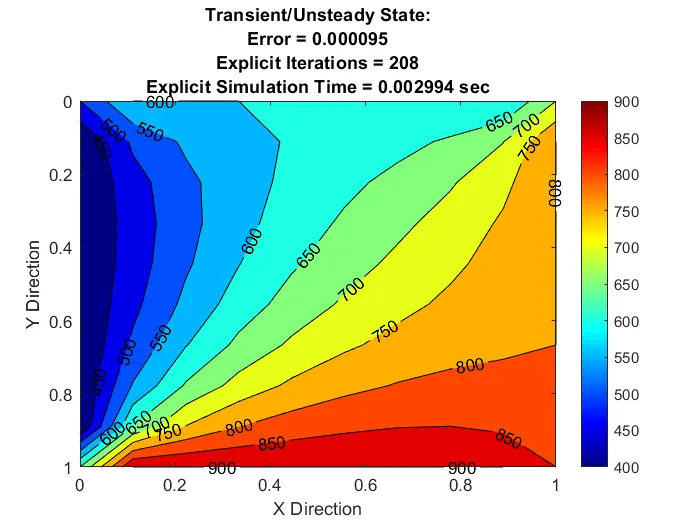
For Transient state or Unsteady state,

a) Explicit

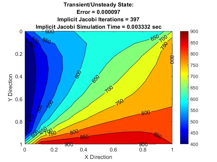
b) Implicit

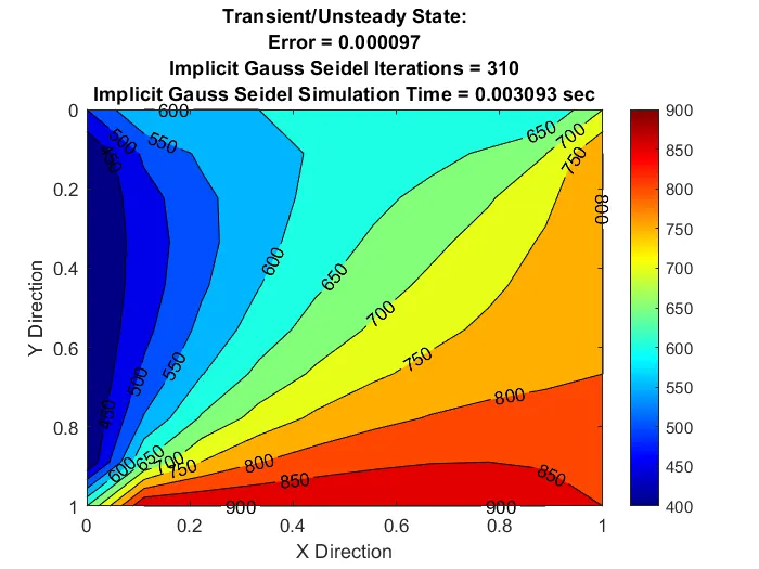
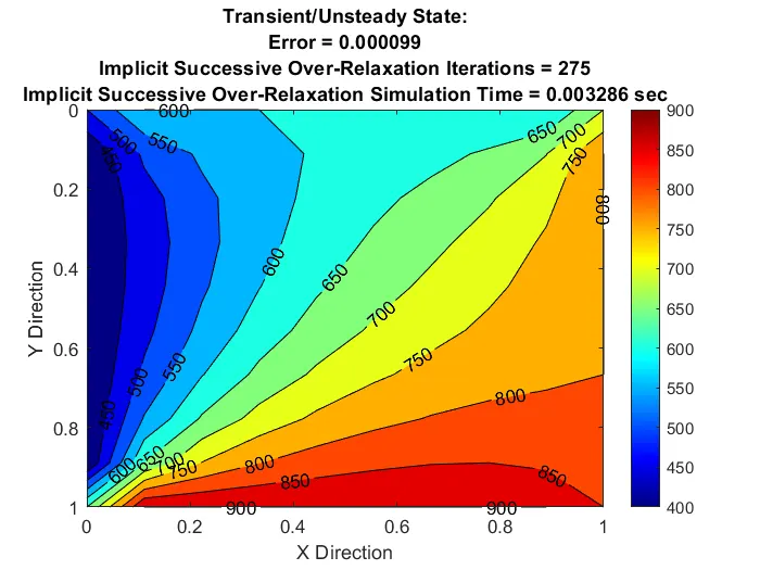
Now, a comparison of Transient or Unsteady state iterative methods.

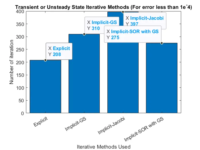
Conclusion:

1. For steady-state iterative methods, Successive Over-Relaxation is best in comparison, followed by Gauss-Seidel. Where the Jacobi method took most iterations to converge.

2. For Unsteady-state iterative methods, Explicit method took less iteration when compared to every Implicit method.

3. For Unsteady-state Implicit iterative methods, Successive Over-Relaxation with Gauss-Seidel is better, followed by Implicit Gauss-Seidel. As usual, Implicit Jacobi method took most iterations to converge.

4. Based on the results, the number of iterations is not always proportional to computational time. (This conclusion may be wrong)