Challenge

Solving the steady and unsteady 2D heat conduction problem

SSaurabh Burde21 Dec 2020

SOLVING THE STEADY AND UNSTEADY 2D HEAT CONDUCTION PROBLEM

Aim

Write a program to solve the 2D heat conduction equation by using the point iterative techniques for given boundary conditions.
Solve above problem for Steady state analysis and Transient state analysis.
Use Jacobi, Gauss-seidel and Successive over-relaxation iterative methods to get the approximations with allowable error 1e-4.
For the transient Analysis, write the code by implementing both implicit and explicit schemes.
Write detailed report explaining overall process and MatLab codes.

Objective

Create Function program for all the iterative solver techniques by giving each method its serial number so that after running main program user just have to type specific number to get answer by particular iteration technique.
Write main program where user can make changes in inputs parameter as per his/her needs.
Specify input line which ask user for the selection of specific iterative techniques, to make it easy,create table which shows each iterative technique and its serial number.
Call the function in main program to run the all the given input parameters from each iterative technique.

2D heat conduction equation

For Steady state Conduction Equation

`(del^2T)/(delx^2)+(del^2T)/(dely^2)=0`

& Transient State Conduction Equation

`(delT)/(delt)+alpha((del^2T)/(delx^2)+(del^2T)/(dely^2))=0`

Firstly, provide all the input parameter in the main program. But before that it is better practice to clear all previous data, clear the command window and close all previous figure windows using following codes and then proceed with providing inputs for the our program.

clear all
close all
clc
 
%% Inputs
%Number of grid points on x and y axis
nx = 10;
ny = 10;
 
% Time step
dt = 1e-2;
  
% Tolerance and dummy error
error = 9e9;
tol = 1e-4;

For boundary condition, the temperature on each side of the is not same so we also have to take average temperature of two adjacent side to get the corner temperature, and temperature inside the boundary consider as 300K.

% let the initial temperature be 300k
t = 300*ones(nx,ny);
 
% Applying Boundary Condition
t(1:end,1)= 400;
t(end,1:end)=900;
t(1,1:end)=600;
t(1:end,end)=800;
 
t(1,1)=(t(1,2)+t(2,1))/2;
t(end,1)=(t(end,2)+t((end-1),1))/2;
t(1,end)=(t(1,(end-1))+t(2,end))/2;
t(end,end)=(t((end-1),(end))+t(end,(end-1)))/2;

Check above if code is correct or not by opening the temperature matrix.

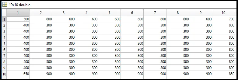
Using above value we will calculate following parameters, which, we going to keep in function program.

% Domain is unit square along x and y 
x = linspace(0,1,nx);
Y = linspace(0,1,ny);

dx = 1/(nx-1);
dy = 1/(ny-1);
 
% Time step
nt = 2/dt;
 
% Stady State analysis
told = t;
t_initial = t;

And for user selection make a list of iterative solver serial vise in the main program. Afterwards, provide input line for the user to select required solver. To process user selection, later call the function by pasting function line and we can also print number of iteration if required using following codes.

fprintf('n              Iteration Methodsn');
fprintf('[1] Steady state analysis using Jacobi methodn');
fprintf('[2] Steady state analysis using Gauss-seidel methodn');
fprintf('[3] Steady state analysis using Successive Over-relaxation methodn');
fprintf('[4] Transient State analysis using Implicit Jacobi methodn');
fprintf('[5] Transient State analysis using Implicit Gauss-seidel methodn');
fprintf('[6] Transient State analysis using Implicit Successive over-relaxation methodn');
fprintf('[7] Transient State analysis using Explicit Jacobi methodn');
fprintf('[8] Transient State analysis using Explicit Gauss-seidel methodn');
fprintf('[9] Transient State analysis using Explicit Successive over-relaxation methodnn');
 
Type_of_solver = input('Select the method of solver from above list = ');
 
[iter]=iter_methods(Type_of_solver,nx,ny,dt,t,error,tol,alpha);
 
fprintf('nNo. of Iteration = %.0fn',iter);

Next, We are going to solve First iteration using Jacobi iteration method. Therefore, lets first understand about Jacobi iterative scheme.

[1] Steady State Conduction using Jacobi iteration solver

Jacobi Iterative method:-

In Jacobi method, we use the value obtained by previous step, meaning, the temperature at n+1^th iteration is found using old values of the temperature defined at n^thiterations. Using the approximation obtained by solving each iteration the computing continued until the desired accuracy of the solution is obtained.

Before we start, our prior step will be to discretise the Steady state conduction equation.

`(del^2T)/(delx^2)+(del^2T)/(dely^2)=0`

By using central difference scheme

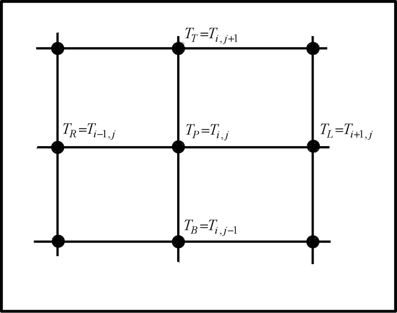
`(T_L-2T_P+T_R)/(Deltax^2) +(T_T-2T_P+T_B)/(Deltay^2) =0`

`(2T_P)/(Deltax^2) +(2T_P)/(Deltay^2)=(T_L+T_R)/(Deltax^2) +(T_T+T_B)/(Deltay^2)`

`T_P(2(Deltax^2+Deltay^2)/(Deltax^2 Deltay^2)) =(T_L+T_R)/(Deltax^2) +(T_T+T_B)/(Deltay^2)`

Put, `(2(Deltax^2+Deltay^2)/(Deltax^2 Deltay^2))=K`

Hence, give import the formula for K in codding.

K=2*(dx^2+dy^2)/((dx^2)*(dy^2));

Then,

`T_P =1/K ((T_L+T_R)/(Deltax^2) +(T_T+T_B)/(Deltay^2))`

Now, we can create iterative loop for the 2D steady state Jacobi solver for nx and ny domin region which value we will provide in main program.

%% Steady State Conduction using jacobi iteration solver
tic
% Loop for type of iterative solver by sr.no.
if Type_of_solver == 1
    iter=1;
    while (error>tol)
        for i = 2:nx-1
            for j = 2:ny-1
                t(i,j)=(1/K)*((told((i-1),j)+told((i+1),j))/(dx^2)+(told(i,(j-1))+told(i,(j+1)))/(dy^2));
            end
        end
        error = max(max(abs(told-t)));
        told=t;
        iter = iter+1;
        
        
        set(gcf,'Position',[100,100,800,650])
        figure(1)
        [X,Y]=contourf(t);
        clabel(X,Y)
        colormap;
        colorbar
        set(gca,'ydir','reverse')
        title('Steady State analysis using Jacobi method','fontsize',18,'fontweight','bold')
        pause(0.001)
    end
    toc;
    saveas(gcf,'Steady State Conduction using jacobi iteration solver.jpg');
end

Output in command window:-

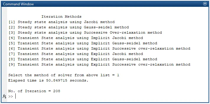
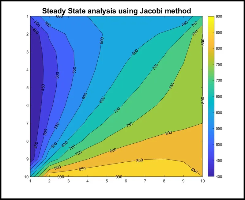
Then program will give us the animated graphical solution for the iterative solver of 2D state Conduction using Jacobi iteration and after the end of loop we will get our final graph saved in .jpg format.

Output final graph from the above codes:-

[2] Steady state temperature using Gauss-Seidal iteration solver

Similar way, we have to write the code for Gauss-seidel method

Gauss-seidel method:-

Gauss-seidel method is an improved from of Jacobi method, also known as the successive displacement method. The difference between the Gauss-seidel and Jacobi methods is that the jacobi method uses the vales obtained from the previous step while the Gauss-Seidel method always applies the latest updated values during the iterative procedures. Which means at n+t^th temperature it uses n+1^th iterations that have already been computed which overwrites old approximate values with new ones.

Therefore, for Steady state 2D Gauss-seidel method just replace told with t and overall program will remain as it is.

%% Steady state temperature using Gauss-Seidal iteration solver
tic
if Type_of_solver == 2
    iter=1;
    while (error>tol)
        for i = 2:nx-1
            for j = 2:ny-1
                t(i,j)=(1/K)*((t((i-1),j)+t((i+1),j))/(dx^2)+(t(i,(j-1))+t(i,(j+1)))/(dy^2));
            end
        end
        error = max(max(abs(told-t)));
        told=t;
        iter = iter+1;
        
        
        set(gcf,'Position',[100,100,800,650])
        figure(1)
        [X,Y]=contourf(t);
        clabel(X,Y)
        colormap;
        colorbar
        set(gca,'ydir','reverse')
        title('Steady state analysis using Gauss-seidel method','fontsize',18,'fontweight','bold')
        pause(0.001)
    end
    toc;
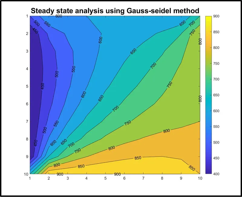
    saveas(gcf,'Steady state analysis using Gauss-seidel method.jpg');
end

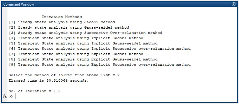
Output of above codes in command window:-

Output plot for Steady state Gauss-seidel Method:-

[3] Steady state temperature using Successive over relaxation iteration solver

Successive over-relaxation solver:-

Iterate methods usually converge to the correct solution from one side, that is, the correction tⁱ⁺¹ - tⁱ stays on the same side of the sign as i increases. This is used by the SOR method to speed up the convergence.

`T_P =(1-omega)T_(old)+omega(1/K ((T_L+T_R)/(Deltax^2) +(T_T+T_B)/(Deltay^2)))`

Successive over relaxation is a variant of the Gauss-seidel method in which `(1-omega)T_(old)+omega(Equation)` is added for acceleration or over-relaxation propose which must be between 1 and 2.

So in programming we will take `omega` as 1.1

For steady state successive method our program format will be same we will just update the formula for method following way.

%% Steady state temperature using Successive over relaxation iteration solver
tic
if Type_of_solver == 3
    iter=1;
    while (error>tol)
        for i = 2:nx-1
            for j = 2:ny-1
                
                t(i,j)=(1/K)*((t((i-1),j)+told((i+1),j))/(dx^2)+(told(i,(j+1))+t(i,(j-1)))/(dy^2));
 
                t(i,j)=(1-omega)*told(i,j)+omega*(t(i,j));
                
            end
        end
        error = max(max(abs(told-t)));
        told=t;
        iter = iter+1;
        
        
        set(gcf,'Position',[100,100,800,650])
        figure(1)
        [X,Y]=contourf(t);
        clabel(X,Y)
        colormap;
        colorbar
        set(gca,'ydir','reverse')
        title('Steady state analysis using Successive Over-relaxation method','fontsize',18,'fontweight','bold')
        pause(0.001)
    end
    toc;
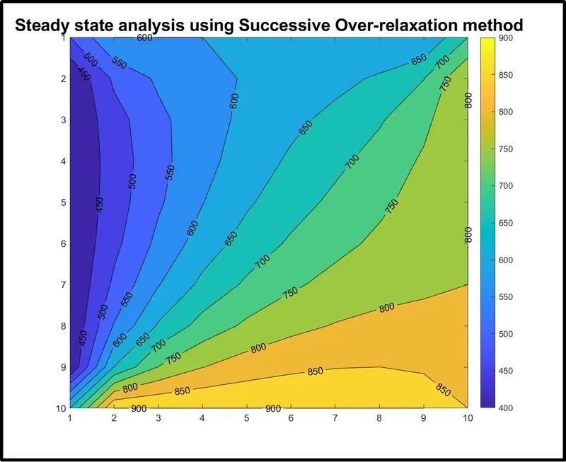
    saveas(gcf,'Steady state analysis using Successive Over-relaxation method.jpg');
end

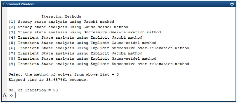
Output for above codes:-

Output graph for steady state successive over relaxation iteration method:-

[4] Transient State analysis using Implicit Jacobi method

Transient State Conduction Equation

`(delT)/(delt)+alpha((del^2T)/(delx^2)+(del^2T)/(dely^2))=0`

Descretise the above equation using central difference scheme and use time marching solution for the time data.

`(T_P^(n+1) -T_P^n)/(DeltaT)+alpha((T_L-2T_P+T_R)/(Deltax^2) +(T_T-2T_P+T_B)/(Deltay^2))=0`

For Transient Implicit Method find out value for`(n+1)`

`T_P^(n+1) =T_P^n +alpha Delta t((T_L-2T_P+T_R)/(Deltax^2) +(T_T-2T_P+T_B)/(Deltay^2))`

Put, `k_1=(alpha Delta t)/(Deltax^2) And k_2=(alpha Delta t)/(Deltay^2)`

`T_P^(n+1) =T_P^n +k_1(T_L^(n+1)-2T_P^(n+1)+T_R^(n+1)) +k_2(T_T^(n+1)-2T_P^(n+1)+T_B^(n+1))`

`T_P^(n+1)-k_1T_L^(n+1)+2k_1T_P^(n+1)-k_1T_R^(n+1)-k_2T_T^(n+1)+2k_2T_P^(n+1)-k_2T_B^(n+1)=T_P^n`

`T_P^(n+1)(1-2K_1+2K_2)-k_1T_L^(n+1)-k_1T_R^(n+1)-k_2T_T^(n+1)-k_2T_B^(n+1)=T_P^n`

`T_P^(n+1)(1-2K_1+2K_2)=T_P^n+k_1T_L^(n+1)+k_1T_R^(n+1)+k_2T_T^(n+1)+k_2T_B^(n+1)`

`T_P^(n+1)(1-2K_1+2K_2)=(1-2K_1+2K_2)(T_P^n+k_1T_L^(n+1)+k_1T_R^(n+1)+k_2T_T^(n+1)+k_2T_B^(n+1))`

Hence, using above equation we will write codes for transient state 2D equation implementing it with, first, Jacobi method for time step nt. We are not considering number of iteration here as we are solving for time steps.

%% Transient State analysis using Implicit Jacobi method
tic
if Type_of_solver == 4
    for nt=1:250
        iter=1;
        error =9e9;
        while(error>tol)
            
            for i=2:nx-1
                for j=2:ny-1
                
                    term0=(1+(2*k1)+(2*k2))^-1;
                    term2=(k1*term0);
                    term3=(k2*term0);
                    term4=(told((i-1),j))+(told((i+1),j));
                    term5=(told(i,(j-1)))+(told(i,(j+1)));
                
                    t(i,j)=(t_initial(i,j)*term0)+(term4*term2)+(term5*term3);
                end
            end
            error=max(max(abs(told-t)));
            told=t;
            iter=iter+1;
        end
        t_initial=told;
        
        set(gcf,'Position',[100,100,800,650])
        figure(1)
        [X,Y]=contourf(t);
        clabel(X,Y)
        colormap;
        colorbar
        set(gca,'ydir','reverse')
        title('Transient State analysis using Implicit Jacobi method','fontsize',18,'fontweight','bold')
        pause(0.001)
    end
    toc;
    saveas(gcf,'Transient State analysis using Implicit Jacobi method.jpg');
end

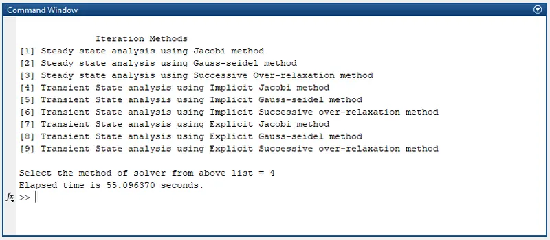
Output for above Codes:-

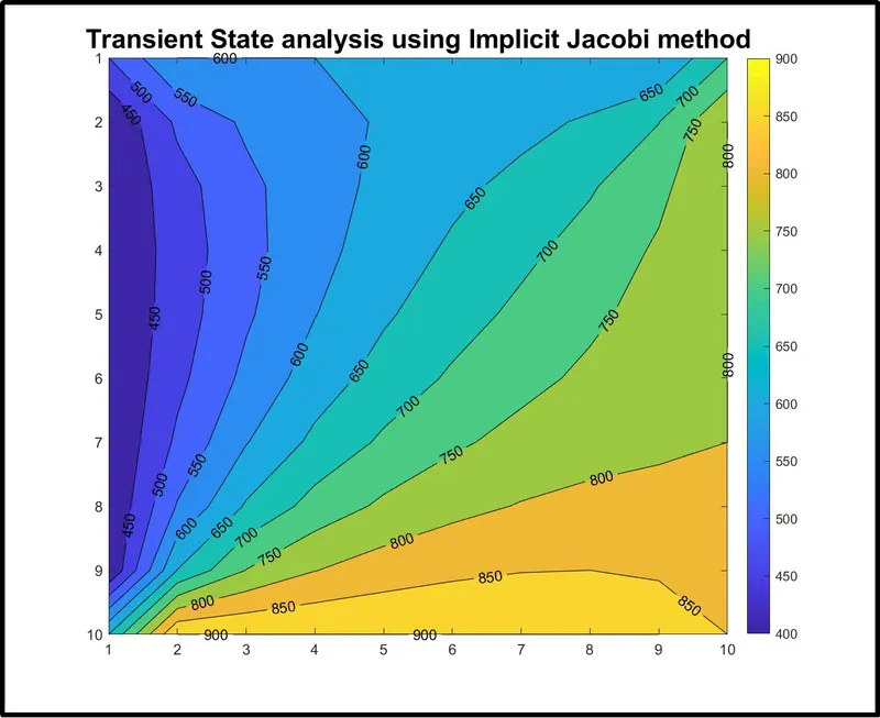
Output plot for the Transient State analysis using implicit Jacobi method:-

[5] Transient State analysis using Implicit Gauss-seidel method

Similarly, we will use same code format for Transient State analysis using Implicit Gauss-seidel method; only change the equation, use temperature at n+t^th temperature as it uses n+1^th iterations that have already been computed which overwrites old approximate values with new ones.

%% Transient State analysis using Implicit Gauss-seidel method
 
tic
if Type_of_solver == 5
    for nt=1:250
        iter=1;
        error =9e9;
        while(error>tol)
            
            for i=2:nx-1
                for j=2:ny-1
                
                    term0=(1+(2*k1)+(2*k2))^-1;
                    term2=(k1*term0);
                    term3=(k2*term0);
                    term4=(t((i-1),j))+(t((i+1),j));
                    term5=(t(i,(j-1)))+(t(i,(j+1)));
                
                    t(i,j)=(t_initial(i,j)*term0)+(term4*term2)+(term5*term3);
                end
            end
            error=max(max(abs(told-t)));
            told=t;
            iter=iter+1;
        end
        t_initial=told;
        
        set(gcf,'Position',[100,100,800,650])
        figure(1)
        [X,Y]=contourf(t);
        clabel(X,Y)
        colormap;
        colorbar
        set(gca,'ydir','reverse')
        title('Transient State analysis using Implicit Gauss-seidel method','fontsize',18,'fontweight','bold')
        pause(0.001)
    end
    toc;
    saveas(gcf,'Transient State analysis using Implicit Gauss-seidel method.jpg');
end

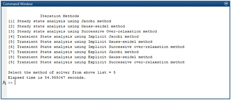
Output for above codes:-

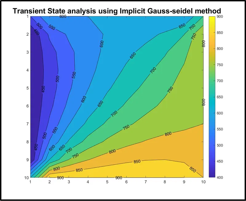
Output plot for above codes:-

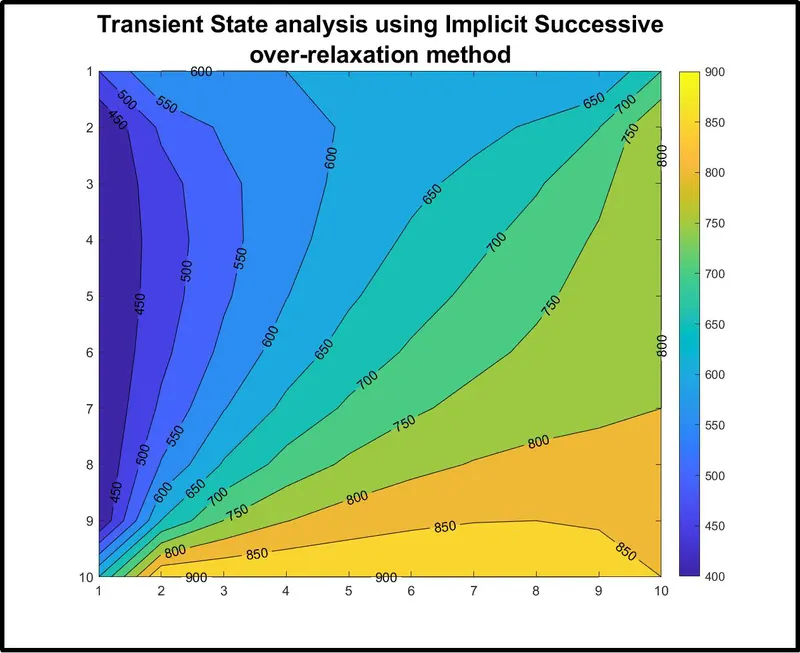
[6]Transient State analysis using Implicit Successive over-relaxation method

using same structure, just adjusting a equation as per Implicit Successive over-relaxation method we will use the codes to calculate results.

%% Transient State analysis using Implicit Successive over-relaxation method
 
tic
if Type_of_solver == 6
    for nt=1:250
        iter=1;
        error =9e9;
        while(error>tol)
            
            for i=2:nx-1
                for j=2:ny-1
                
                    term0=(1+(2*k1)+(2*k2))^-1;
                    term2=(k1*term0);
                    term3=(k2*term0);
                    term4=(t((i-1),j))+(t((i+1),j));
                    term5=(t(i,(j-1)))+(t(i,(j+1)));
                
                    t(i,j)=omega*((t_initial(i,j)*term0)+(term4*term2)+(term5*term3))-(omega-1)*t_initial(i,j);
                end
            end
            error=max(max(abs(told-t)));
            told=t;
            iter=iter+1;
        end
        t_initial=told;
        
        set(gcf,'Position',[100,100,800,650])
        figure(1)
        [X,Y]=contourf(t);
        clabel(X,Y)
        colormap;
        colorbar
        set(gca,'ydir','reverse')
        title({'Transient State analysis using Implicit Successive';'over-relaxation method'},'fontsize',18,'fontweight','bold')
        pause(0.001)
    end
    toc;
    saveas(gcf,'Transient State analysis using Implicit Successive over-relaxation method.jpg');
end

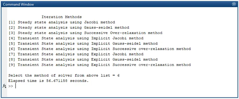
Output for above codes:-

Output plot for above codes:-

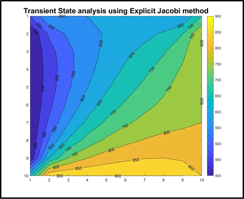
[7] Transient State analysis using Explicit Jacobi method

next, for explicit method we will use direct transient Discretise equation

`T_P^(n+1) =T_P^n +k_1(T_L^(n+1)-2T_P^(n+1)+T_R^(n+1)) +k_2(T_T^(n+1)-2T_P^(n+1)+T_B^(n+1))`

Using above equation we can now write following program

%% Transient State analysis using Explicit Jacobi method
tic
if Type_of_solver == 7
    iter=1;
    while (error>tol)
        for i = 2:nx-1
            for j = 2:ny-1
                
                term1=told(i,j);
                term2=(told(i-1,j)-2*told(i,j)+told(i+1,j));
                term3=(told(i,j-1)-2*told(i,j)+told(i,j+1));
                
                t(i,j)=term1+k1*term2+k2*term3;
            end
        end
        error = max(max(abs(told-t)));
        told=t;
        iter = iter+1;
        
        
        set(gcf,'Position',[100,100,800,650])
        figure(1)
        [X,Y]=contourf(t);
        clabel(X,Y)
        colormap;
        colorbar
        set(gca,'ydir','reverse')
        title('Transient State analysis using Explicit Jacobi method','fontsize',18,'fontweight','bold')
        pause(0.001)
    end
    toc;
    saveas(gcf,'Transient State analysis using Explicit Jacobi method.jpg');
end

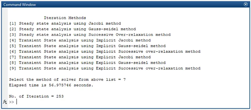
Output for the code

Output plot for above codes

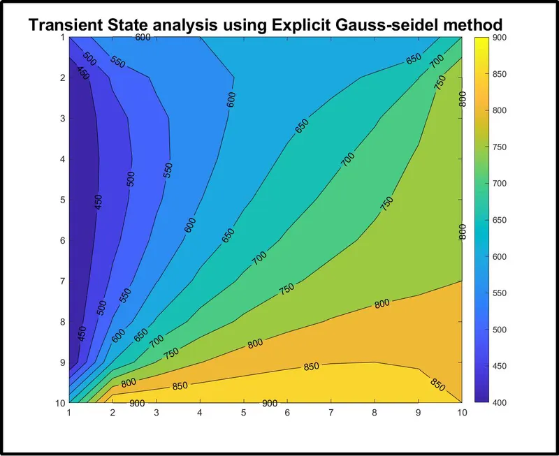
[8] Transient State analysis using Explicit Gauss-seidel method

Same technique we will use to solve Explicit Gauss-seidel method

%% Transient State analysis using Explicit Gauss-seidel method
tic
if Type_of_solver == 8
    iter=1;
    while (error>tol)
        for i = 2:nx-1
            for j = 2:ny-1
                
                term1=told(i,j);
                term2=(t(i-1,j)-2*t(i,j)+t(i+1,j));
                term3=(t(i,j-1)-2*t(i,j)+t(i,j+1));
                t(i,j)=term1+k1*term2+k2*term3;
                
            end
        end
        error = max(max(abs(told-t)));
        told=t;
        iter = iter+1;
        
        
        set(gcf,'Position',[100,100,800,650])
        figure(1)
        [X,Y]=contourf(t);
        clabel(X,Y)
        colormap;
        colorbar
        set(gca,'ydir','reverse')
        title('Transient State analysis using Explicit Gauss-seidel method','fontsize',18,'fontweight','bold')
        pause(0.001)
    end
    toc;
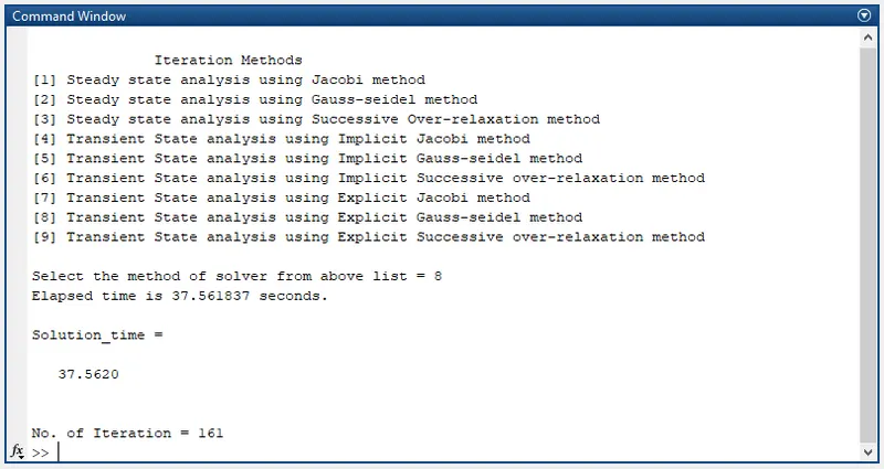
    Solution_time =toc
    saveas(gcf,'Transient State analysis using Explicit Gauss-seidel method.jpg');
end

Output of above codes

Output Graph of the program:-

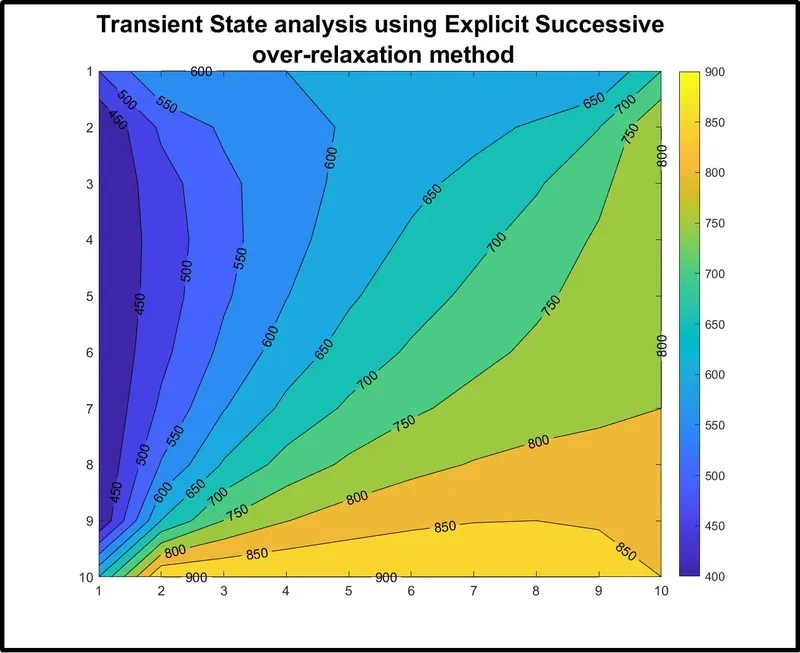
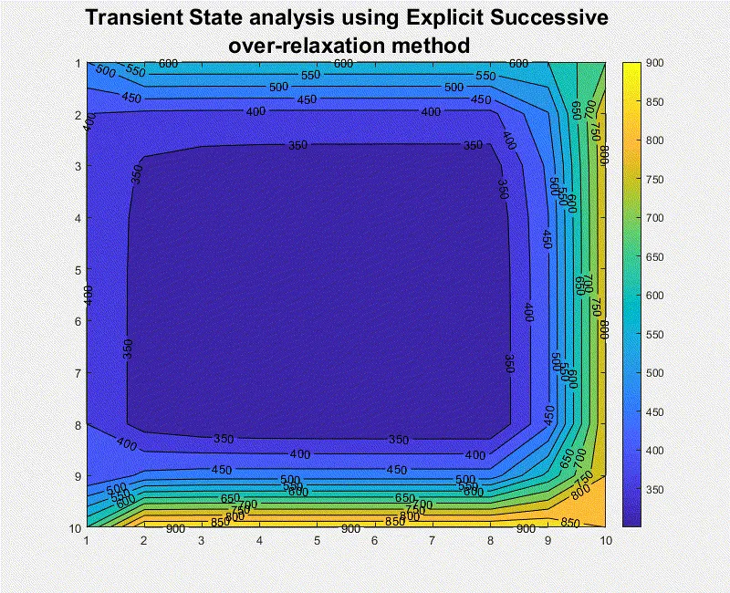
[9] Transient State analysis using Explicit Successive over-relaxation method

Finally, use same structure to get results for Explicit Successive over-relaxation method.

%% Explicit temperature using Successive over relaxation iteration solver
tic
if Type_of_solver == 9
    iter=1;
    while (error>tol)
        for i = 2:nx-1
            for j = 2:ny-1
                
                term1=told(i,j);
                term2=(t(i-1,j)-2*t(i,j)+t(i+1,j));
                term3=(t(i,j-1)-2*t(i,j)+t(i,j+1));
                t(i,j)=omega*(term1+k1*term2+k2*term3)-(omega-1)*term1;
                
            end
        end
        error = max(max(abs(told-t)));
        told=t;
        iter = iter+1;
        
        
        set(gcf,'Position',[100,100,800,650])
        figure(1)
        [X,Y]=contourf(t);
        clabel(X,Y)
        colormap;
        colorbar
        set(gca,'ydir','reverse')
        title('Transient State analysis using Explicit Successive over-relaxation method','fontsize',18,'fontweight','bold')
        pause(0.001)
    end
    toc;
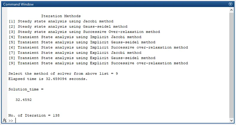
    Solution_time =toc
    saveas(gcf,'Transient State analysis using Explicit Successive over-relaxation method.jpg');
end

Output for above codes

Output chart for Transient Explicit Successive over-relaxation method:-

Conclusion

Compete over view on the hypothesis conclude that all the method are useful to converge the solution but the step its take to converge it are very different.

For steady state analysis, Jacobi method take 208, where Gauss-siedel method take-120 and if we look at the Successive Over-relaxation method it only 98 to converge the solution. Selection of proper technique is very important to reduce computation time.

Therefore, in terms of converging solution with minimum iteration the Successive over-relaxation scheme is the most effective which provide solution in minimum iteration even with Transient implicit and transient explicit method.

Animation.Gif file

Complete Main Program

clear all
close all
clc

% Given Conditions
nx = 10;
ny = 10;


% Time step
dt = 1e-2;

% let the initial temperature be 300k
t = 300*ones(nx,ny);

% Applying Boundary Condition
t(1:end,1)= 400;
t(end,1:end)=900;
t(1,1:end)=600;
t(1:end,end)=800;

t(1,1)=(t(1,2)+t(2,1))/2;
t(end,1)=(t(end,2)+t((end-1),1))/2;
t(1,end)=(t(1,(end-1))+t(2,end))/2;
t(end,end)=(t((end-1),(end))+t(end,(end-1)))/2;

% Tolerance and error
error = 9e9;
tol = 1e-4;

%
alpha = 0.25;

% Omega value for successive Over relaxation
omega = 1.1;

fprintf('n              Iteration Methodsn');
fprintf('[1] Steady state analysis using Jacobi methodn');
fprintf('[2] Steady state analysis using Gauss-seidel methodn');
fprintf('[3] Steady state analysis using Successive Over-relaxation methodn');
fprintf('[4] Transient State analysis using Implicit Jacobi methodn');
fprintf('[5] Transient State analysis using Implicit Gauss-seidel methodn');
fprintf('[6] Transient State analysis using Implicit Successive over-relaxation methodn');
fprintf('[7] Transient State analysis using Explicit Jacobi methodn');
fprintf('[8] Transient State analysis using Explicit Gauss-seidel methodn');
fprintf('[9] Transient State analysis using Explicit Successive over-relaxation methodnn');


Type_of_solver = input('Select the method of solver from above list = ');

[iter]=iter_methods(Type_of_solver,nx,ny,dt,t,error,tol,alpha,omega);

fprintf('nNo. of Iteration = %.0fn',iter);

Complete Function Program

function [iter]=iter_methods(Type_of_solver,nx,ny,dt,t,error,tol,alpha,omega)


% Domain is unit square along x and y 
x = linspace(0,1,nx);
Y = linspace(0,1,ny);


dx = 1/(nx-1);
dy = 1/(ny-1);

% Time step
nt = 2/dt;

% Stady State analysis
told = t;
t_initial = t;

K=2*(dx^2+dy^2)/((dx^2)*(dy^2));


k1 = alpha*(dt/(dx^2));
k2 = alpha*(dt/(dy^2));

%% Steady State Conduction using jacobi iteration solver
tic
% Loop for type of iterative solver by sr.no.
if Type_of_solver == 1
    iter=1;
    while (error>tol)
        for i = 2:nx-1
            for j = 2:ny-1
                t(i,j)=(1/K)*((told((i-1),j)+told((i+1),j))/(dx^2)+(told(i,(j-1))+told(i,(j+1)))/(dy^2));
            end
        end
        error = max(max(abs(told-t)));
        told=t;
        iter = iter+1;
        
        
        set(gcf,'Position',[100,100,800,650])
        figure(1)
        [X,Y]=contourf(t);
        clabel(X,Y)
        colormap;
        colorbar
        set(gca,'ydir','reverse')
        title('Steady State analysis using Jacobi method','fontsize',18,'fontweight','bold')
        pause(0.001)
    end
    toc;
    saveas(gcf,'Steady State Conduction using jacobi iteration solver.jpg');
end



%% Steady state temperature using Gauss Seidal iteration solver
tic
if Type_of_solver == 2
    iter=1;
    while (error>tol)
        for i = 2:nx-1
            for j = 2:ny-1
                t(i,j)=(1/K)*((t((i-1),j)+t((i+1),j))/(dx^2)+(t(i,(j-1))+t(i,(j+1)))/(dy^2));
            end
        end
        error = max(max(abs(told-t)));
        told=t;
        iter = iter+1;
        
        
        set(gcf,'Position',[100,100,800,650])
        figure(1)
        [X,Y]=contourf(t);
        clabel(X,Y)
        colormap;
        colorbar
        set(gca,'ydir','reverse')
        title('Steady state analysis using Gauss-seidel method','fontsize',18,'fontweight','bold')
        pause(0.001)
    end
    toc;
    saveas(gcf,'Steady state analysis using Gauss-seidel method.jpg');
end  



%% Steady state temperature using Successive over relaxation iteration solver
tic
if Type_of_solver == 3
    iter=1;
    while (error>tol)
        for i = 2:nx-1
            for j = 2:ny-1
                
                t(i,j)=(1/K)*((t((i-1),j)+told((i+1),j))/(dx^2)+(told(i,(j+1))+t(i,(j-1)))/(dy^2));

                t(i,j)=(1-omega)*told(i,j)+omega*(t(i,j));
                
            end
        end
        error = max(max(abs(told-t)));
        told=t;
        iter = iter+1;
        
        
        set(gcf,'Position',[100,100,800,650])
        figure(1)
        [X,Y]=contourf(t);
        clabel(X,Y)
        colormap;
        colorbar
        set(gca,'ydir','reverse')
        title('Steady state analysis using Successive Over-relaxation method','fontsize',18,'fontweight','bold')
        pause(0.001)
    end
    toc;
    saveas(gcf,'Steady state analysis using Successive Over-relaxation method.jpg');
end



        

%% Transient State analysis using Implicit Jacobi method
tic
if Type_of_solver == 4
    for nt=1:250
        iter=1;
        error =9e9;
        while(error>tol)
            
            for i=2:nx-1
                for j=2:ny-1
                
                    term0=(1+(2*k1)+(2*k2))^-1;
                    term2=(k1*term0);
                    term3=(k2*term0);
                    term4=(told((i-1),j))+(told((i+1),j));
                    term5=(told(i,(j-1)))+(told(i,(j+1)));
                
                    t(i,j)=(t_initial(i,j)*term0)+(term4*term2)+(term5*term3);
                end
            end
            error=max(max(abs(told-t)));
            told=t;
            iter=iter+1;
        end
        t_initial=told;
        
        set(gcf,'Position',[100,100,800,650])
        figure(1)
        [X,Y]=contourf(t);
        clabel(X,Y)
        colormap;
        colorbar
        set(gca,'ydir','reverse')
        title('Transient State analysis using Implicit Jacobi method','fontsize',18,'fontweight','bold')
        pause(0.001)
    end
    toc;
    saveas(gcf,'Transient State analysis using Implicit Jacobi method.jpg');
end



%% Transient State analysis using Implicit Gauss-seidel method

tic
if Type_of_solver == 5
    for nt=1:250
        iter=1;
        error =9e9;
        while(error>tol)
            
            for i=2:nx-1
                for j=2:ny-1
                
                    term0=(1+(2*k1)+(2*k2))^-1;
                    term2=(k1*term0);
                    term3=(k2*term0);
                    term4=(t((i-1),j))+(t((i+1),j));
                    term5=(t(i,(j-1)))+(t(i,(j+1)));
                
                    t(i,j)=(t_initial(i,j)*term0)+(term4*term2)+(term5*term3);
                end
            end
            error=max(max(abs(told-t)));
            told=t;
            iter=iter+1;
        end
        t_initial=told;
        
        set(gcf,'Position',[100,100,800,650])
        figure(1)
        [X,Y]=contourf(t);
        clabel(X,Y)
        colormap;
        colorbar
        set(gca,'ydir','reverse')
        title('Transient State analysis using Implicit Gauss-seidel method','fontsize',18,'fontweight','bold')
        pause(0.001)
    end
    toc;
    saveas(gcf,'Transient State analysis using Implicit Gauss-seidel method.jpg');
end




%% Transient State analysis using Implicit Successive over-relaxation method

tic
if Type_of_solver == 6
    for nt=1:250
        iter=1;
        error =9e9;
        while(error>tol)
            
            for i=2:nx-1
                for j=2:ny-1
                
                    term0=(1+(2*k1)+(2*k2))^-1;
                    term2=(k1*term0);
                    term3=(k2*term0);
                    term4=(t((i-1),j))+(t((i+1),j));
                    term5=(t(i,(j-1)))+(t(i,(j+1)));
                
                    t(i,j)=omega*((t_initial(i,j)*term0)+(term4*term2)+(term5*term3))-(omega-1)*t_initial(i,j);
                end
            end
            error=max(max(abs(told-t)));
            told=t;
            iter=iter+1;
        end
        t_initial=told;
        
        set(gcf,'Position',[100,100,800,650])
        figure(1)
        [X,Y]=contourf(t);
        clabel(X,Y)
        colormap;
        colorbar
        set(gca,'ydir','reverse')
        title({'Transient State analysis using Implicit Successive';'over-relaxation method'},'fontsize',18,'fontweight','bold')
        pause(0.001)
    end
    toc;
    saveas(gcf,'Transient State analysis using Implicit Successive over-relaxation method.jpg');
end



%% Transient State analysis using Explicit Jacobi method
tic
if Type_of_solver == 7
    iter=1;
    while (error>tol)
        for i = 2:nx-1
            for j = 2:ny-1
                
                term1=told(i,j);
                term2=(told(i-1,j)-2*told(i,j)+told(i+1,j));
                term3=(told(i,j-1)-2*told(i,j)+told(i,j+1));
                
                t(i,j)=term1+k1*term2+k2*term3;
            end
        end
        error = max(max(abs(told-t)));
        told=t;
        iter = iter+1;
        
        
        set(gcf,'Position',[100,100,800,650])
        figure(1)
        [X,Y]=contourf(t);
        clabel(X,Y)
        colormap;
        colorbar
        set(gca,'ydir','reverse')
        title('Transient State analysis using Explicit Jacobi method','fontsize',18,'fontweight','bold')
        pause(0.001)
    end
    toc;
    saveas(gcf,'Transient State analysis using Explicit Jacobi method.jpg');
end




%% Transient State analysis using Explicit Gauss-seidel method
tic
if Type_of_solver == 8
    iter=1;
    while (error>tol)
        for i = 2:nx-1
            for j = 2:ny-1
                
                term1=told(i,j);
                term2=(t(i-1,j)-2*t(i,j)+t(i+1,j));
                term3=(t(i,j-1)-2*t(i,j)+t(i,j+1));
                t(i,j)=term1+k1*term2+k2*term3;
                
            end
        end
        error = max(max(abs(told-t)));
        told=t;
        iter = iter+1;
        
        
        set(gcf,'Position',[100,100,800,650])
        figure(1)
        [X,Y]=contourf(t);
        clabel(X,Y)
        colormap;
        colorbar
        set(gca,'ydir','reverse')
        title('Transient State analysis using Explicit Gauss-seidel method','fontsize',18,'fontweight','bold')
        pause(0.001)
    end
    toc;
    Solution_time =toc
    saveas(gcf,'Transient State analysis using Explicit Gauss-seidel method.jpg');
end



%% Explicit temperature using Successive over relaxation iteration solver
tic
if Type_of_solver == 9
    iter=1;
    while (error>tol)
        for i = 2:nx-1
            for j = 2:ny-1
                
                term1=told(i,j);
                term2=(t(i-1,j)-2*t(i,j)+t(i+1,j));
                term3=(t(i,j-1)-2*t(i,j)+t(i,j+1));
                t(i,j)=omega*(term1+k1*term2+k2*term3)-(omega-1)*term1;
                
            end
        end
        error = max(max(abs(told-t)));
        told=t;
        iter = iter+1;
        
        
        set(gcf,'Position',[100,100,800,650])
        figure(1)
        [X,Y]=contourf(t);
        clabel(X,Y)
        colormap;
        colorbar
        set(gca,'ydir','reverse')
        title({'Transient State analysis using Explicit Successive';' over-relaxation method'},'fontsize',18,'fontweight','bold')
        pause(0.001)
    end
    toc;
    Solution_time =toc
    saveas(gcf,'Transient State analysis using Explicit Successive over-relaxation method.jpg');

end   
       
end

Solving the steady and unsteady 2D heat conduction problem

SOLVING THE STEADY AND UNSTEADY 2D HEAT CONDUCTION PROBLEM

Ship work like this
in your own course.

Talk to a career counsellor

SOLVING THE STEADY AND UNSTEADY 2D HEAT CONDUCTION PROBLEM

Ship work like thisin your own course.

Talk to a career counsellor

Ship work like this
in your own course.