Week 5 - Mid term project - Solving the steady and unsteady 2D heat conduction problem

Aim:To Solve the 2D heat conduction equation by using the point iterative techniques.

Inputs we have assumed here

L=1

nx=20

ny=nx

error criteria is 1e-4

The Boundary conditions for the problem are as follows;

Top Boundary = 600 K

Bottom Boundary = 900 K

Left Boundary = 400 K

Right Boundary = 800 K

Techniques or methods we are using :

1. Jacobi

2. Gauss-seidel

3. Successive over-relaxation

Steady state solution:

``(delta^2T)/(deltax^2)+(delta^2T)/(deltay^2)=0`

Discretizing the above equation:

`(delta^2T)/(deltax^2)=(Ti-1,j-2Ti,j+Ti+1,j)/(Deltax^2`

`(delta^2T)/(deltay^2)=(Ti,j-1-2Ti,j+Ti,j+1)/(Deltay^2`

As we consider nx=ny,Deltax=Deltay

Then rearranging the term we get the equation like this,

`Ti,j=1/4(Ti-1,j+Ti+1,j+Ti,j-1+Ti,j+1`

Coding:

% solving the steady 2D heat conduction problem
close all
clear all
clc

%inputs
L=1; %length of domain and it is a square
%nx,ny no of grid points
nx=30;
ny=nx;
x=linspace(0,1,nx);
y=linspace(0,1,ny);
dx=x(2)-x(1);
dy=y(2)-y(1);
error=9e9;
tol=1e-4;

%define boundary conditions

T_L=400;
T_R=800;
T_T=600;
T_B=900;

T=ones(nx,ny);

%calculation of relaxation factor
omega=2/(1+sin(pi*dx));

% temperature at boundary conditions
   T(:,1)=T_L;
   T(:,end)=T_R;
   T(end,:)=T_T;
   T(1,:)=T_B;
   
 %creating a copy of T
 [X Y]=meshgrid(x,y);
 Told=T;
 
 % jacobi method
 for iterative_solver=1;
     tic
    if iterative_solver==1;
        
        jacobi_iterations=1;
         while (error >tol)
             for i=2:nx-1
                 for j=2:ny-1
                     T(i,j)=0.25*(Told(i-1,j)+Told(i+1,j)+Told(i,j-1)+Told(i,j+1));
                 end
             end
             error=max(max(abs(Told-T)));
             Told=T;
             jacobi_iterations = jacobi_iterations+1;
         end
    end
    F=toc;
    
    %plotting
    figure(1);
    [P,Q]=contourf(X,Y,T);
    clabel(P,Q);
    colormap(jet);
    colorbar;
    title_text=sprintf('Jacobi method,Iteration number=%d,computation time F=%fs',jacobi_iterations,F);
    title(title_text);
    xlabel('Xaxis');
    ylabel('Yaxis');
    fprintf('jacobi=%d/n',jacobi_iterations);
    pause(0.03);
 end
                     
    % for GS method
    for iterative_solver=2;
        % update values
    L=1; %length of domain and it is a square
%nx,ny no of grid points
nx=30;
ny=nx;
x=linspace(0,1,nx);
y=linspace(0,1,ny);
dx=x(2)-x(1);
dy=y(2)-y(1);
error=9e9;
tol=1e-4;

%define boundary conditions

T_L=400;
T_R=800;
T_T=600;
T_B=900;

T=298*ones(nx,ny);

%calculation of relaxation factor
omega=2/(1+sin(pi*dx));

% temperature at boundary conditions
   T(:,1)=T_L;
   T(:,end)=T_R;
   T(end,:)=T_T;
   T(1,:)=T_B;
   
 %creating a copy of T
 [X Y]=meshgrid(x,y);
 Told=T;
 tic;
 

    if iterative_solver==2;
        
        gs_iterations=1;
         while (error >tol)
             for i=2:nx-1
                 for j=2:ny-1
                     T(i,j)=0.25*(T(i-1,j)+Told(i+1,j)+T(i,j-1)+Told(i,j+1));
                 end
             end
             error=max(max(abs(Told-T)));
             Told=T;
             gs_iterations = gs_iterations+1;
         end
    end
    F=toc;
    
    %plotting
    figure(2);
    [P,Q]=contourf(X,Y,T);
    clabel(P,Q);
    colormap(jet);
    colorbar;
    title_text=sprintf('Gauss seidal method,Iteration number=%d,computation time F=%fs',gs_iterations,F);
    title(title_text);
    xlabel('Xaxis');
    ylabel('Yaxis');
    fprintf('gs=%d/n',gs_iterations);
    pause(0.03);
    end
 
    
    
   %SOR
   for iterative_solver=3;
       %update values
       
  L=1; %length of domain and it is a square
%nx,ny no of grid points
nx=30;
ny=nx;
x=linspace(0,1,nx);
y=linspace(0,1,ny);
dx=x(2)-x(1);
dy=y(2)-y(1);
error=9e9;
tol=1e-4;

%define boundary conditions

T_L=400;
T_R=800;
T_T=600;
T_B=900;

T=ones(nx,ny);

%calculation of relaxation factor
omega=2/(1+sin(pi*dx));

% temperature at boundary conditions
   T(:,1)=T_L;
   T(:,end)=T_R;
   T(end,:)=T_T;
   T(1,:)=T_B;
   
 %creating a copy of T
 [X Y]=meshgrid(x,y);
 Told=T;
 tic;
 

    if iterative_solver==3;
        
        SOR_iterations=1;
         while (error >tol)
             for i=2:nx-1
                 for j=2:ny-1
                     T(i,j)=((1-omega)*Told(i,j)+(omega*0.25*(T(i-1,j)+Told(i+1,j)+T(i,j-1)+Told(i,j+1))));
                     
                 end
             end
             error=max(max(abs(Told-T)));
             Told=T;
             SOR_iterations = SOR_iterations+1;
         end
    end
    F=toc;
    
    %plotting
    figure(3);
    [P,Q]=contourf(X,Y,T);
    clabel(P,Q);
    colormap(jet);
    colorbar;
    title_text=sprintf('SOR method,Iteration number=%d,computation time F=%fs',SOR_iterations,F);
    title(title_text);
    xlabel('Xaxis');
    ylabel('Yaxis');
    fprintf('SOR=%d/n',SOR_iterations);
    pause(0.03);
    end

Plottings:

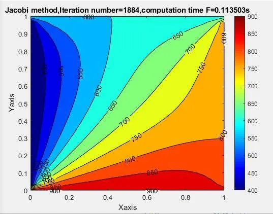
Jacobi method:

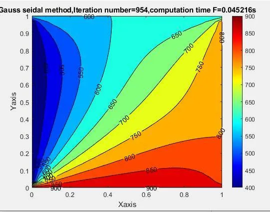
Gauss seidal method:

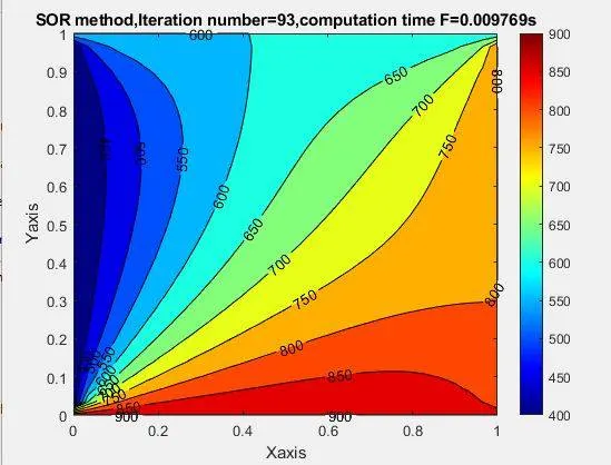
SOR method:

Results:

By comparing above plots that is jacobi,gs & sor method, sor method is solving faster with less iterations and compution time when compared to two other methds.

SOR is taking 93 iterations and computation time =0.009769s

Gauss seidal is taking 954 iterations and computation time=0.04521s

Jacobi method is taking 1884 iterations and comupation time=0.11530s

Transient method:

2-D heat equation for unsteady state is given by:

`aplha(delta^2T)/(deltax^2)+(delta^2T)/(deltay^2)=(deltaT)/(deltat)`

Discretizing the spacial terms:

we get,

`(delta^2T)/(deltax^2)=(Ti-1,j-2Ti,j+Ti+1,j)/(Deltax^2)`

`(delta^2T)/(deltay^2)=(Ti,j-1 -2Ti,j+Ti,j+1)/(Deltay^2)`

Discretizing the time derivative,

`(deltaT)/(deltat)=((T^n+1)i,j-T^ni,j)/(Deltat)`

So now equations become,

for explicit method:

`(T^n+1)i,j=lambda(T^n)i-1,j+(T^n)i,j-1)+[1-4lambda(T^n)i,j+lambda(T^n)i+1,j+(T^n)i,j+1)`

where `lambda=(alphaDeltat)/(Deltax^2)`

lambda is also called as the CFL number ,CFL number is used to check the stability of the solution.

alpha is the convective coefficient.

Code for explicit method:

% solving the steady 2d transient unsteady state heat conduction problem
% explicit
clear all
close all
clc

 L=1; %length of domain and it is a square
%nx,ny no of grid points
nx=51;
ny=nx;
x=linspace(0,L,nx);
y=linspace(0,L,ny);
dx=x(2)-x(1);
dy=y(2)-y(1);
error=9e9;
tol=1e-4;
dt=0.1;
alpha = 1e-3; %convective coefficient
t=200;

%CFL number
M = alpha*dt/(dx^2);


%define boundary conditions

T_L=400;
T_R=800;
T_T=600;
T_B=900;

T=298*ones(nx,ny);


% temperature at boundary conditions
   T(:,1)=T_L;
   T(:,end)=T_R;
   T(end,:)=T_T;
   T(1,:)=T_B;
   
   %calculation of temperature distribution explicity using iterative
   %solvers
   k1=(alpha*dt)/(dx^2);
   k2=(alpha*dt)/(dy^2);
   
   %creating a copy of T
   [X Y]=meshgrid(x,y);
   Told=T;
   nt=t/dt;
   
   %2d transient unsteady state heat conduction equation in explicit method
 
   tic;
  
   for v=1:nt
      
       for i=2:nx-1
               for j=2:ny-1
                   term1=Told(i,j);
                   term2=k1*(Told(i+1,j)-2*Told(i,j)+Told(i-1,j));
                    term3=k2*(Told(i,j+1)-2*Told(i,j)+Told(i,j-1));
                    T(i,j)=term1+term2+term3;
               end
       end

          Told=T;
              
           
   end
       time=toc;
       
       
   
    %plottings
       
     figure(1);
        
    [P,Q] = contourf(X,Y,T);
    clabel(P,Q,"fontsize",12);
    colormap(jet);
    colorbar;
    title_text=sprintf('Explicit method,computation time =%fs,M=%f',time,M');
    title(title_text);
    xlabel('Xaxis');
    ylabel('Yaxis');
    
    pause(0.03);

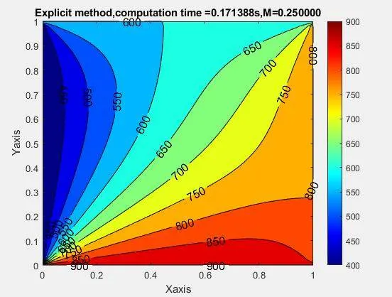
Plottings:

For implicit method:

we know that

`T^(n+1)p=(T^np+k1(T^(n+1)L+T^(n+1)R)+K2(T^(n+1)T+T^(n+1)B))/(1+2k1+2k2`

Code for implicit method:

% solving the steady 2d transient unsteady state heat conduction problem
% implicit
clear all
close all
clc

 L=1; %length of domain and it is a square
%nx,ny no of grid points
nx=20;
ny=nx;
x=linspace(0,L,nx);
y=linspace(0,L,ny);
dx=x(2)-x(1);
dy=y(2)-y(1);
error=9e9;
tol=1e-4;
dt=0.1;
alpha = 1; %convective coefficient
t=200;

%CFL number
M = alpha*dt/(dx^2);


%define boundary conditions

T_L=400;
T_R=800;
T_T=600;
T_B=900;

T=298*ones(nx,ny);


% temperature at boundary conditions
   T(:,1)=T_L;
   T(:,end)=T_R;
   T(end,:)=T_T;
   T(1,:)=T_B;
   
   %calculation of temperature distribution explicity using iterative
   %solvers
   k1=(alpha*dt)/(dx^2);
   k2=(alpha*dt)/(dy^2);
   nt=t/dt;
   %creating a copy of T
   [X Y]=meshgrid(x,y);
   Told=T;
   T_prev_dt=Told;
   
   %2d transient unsteady state heat conduction equation in explicit method
   nt=t/dt;
   iterative_solver=1;
   tic;
   jacobi_iterations=1;
   for v=1:nt
       if iterative_solver==1
           term1=(1+2*k1+2*k2)^(-1);
           term2=k1*term1;
           term3=k2*term1;
           
           error=100;
           while(error >tol)
               for i=2:nx-1
                   for j=2:ny-1
                       H=(Told(i-1,j)+Told(i+1,j));
                       V=(Told(i,j-1)+Told(i,j+1));
                        T(i,j)=(T_prev_dt(i,j)*term1)+(H*term2)+(V*term3);
                   end
               end
               error=max(max(abs(Told-T)));
               Told=T;
               
               jacobi_iterations=jacobi_iterations+1;
           end
           
           T_prev_dt=T;
       end
       time=toc;
       
       %plottings
       
        figure(1);
        
    [P,Q] = contourf(X,Y,T);
    clabel(P,Q,"fontsize",12);
    colormap(jet);
    colorbar;
    title_text=sprintf('Jacobi method,Iteration number=%d,computation time =%fs,M=%f',jacobi_iterations,time,M');
    title(title_text);
    xlabel('Xaxis');
    ylabel('Yaxis');
    
    pause(0.03);
   end
    
   
%    %for gs method
    
    L=1; %length of domain and it is a square
 %nx,ny no of grid points
 nx=20;
 ny=nx;
 x=linspace(0,L,nx);
 y=linspace(0,L,ny);
 dx=x(2)-x(1);
 dy=y(2)-y(1);
 
 error=9e9;
 tol=1e-4;
 dt=0.1;
 alpha = 1; %convective coefficient
 t=200;

% %CFL number
 M = alpha*dt/(dx^2);
 
 
 %define boundary conditions

 T_L=400;
 T_R=800;
 T_T=600;
 T_B=900;
 
 T=298*ones(nx,ny);
 
 
 % temperature at boundary conditions
    T(:,1)=T_L;
    T(:,end)=T_R;
    T(end,:)=T_T;
    T(1,:)=T_B;
    
%    %calculation of temperature distribution explicity using iterative
    %solvers
    k1=(alpha*dt)/(dx^2);
    k2=(alpha*dt)/(dy^2);
    nt=t/dt;
    
%    %creating a copy of T
    [X Y]=meshgrid(x,y);
    Told=T;
    T_prev_dt=Told;
   
%    %2d transient unsteady state heat conduction equation in explicit method
    
   iterative_solver=2;
   tic;
    gs_iterations=1;
    for w=1:nt
       if iterative_solver==2
            term1=(1+2*k1+2*k2)^(-1);
            term2=k1*term1;
            term3=k2*term1;
            
           error=100;
            while(error >tol)
                for i=2:nx-1
                    for j=2:ny-1
                        H=(T(i-1,j)+Told(i+1,j));
                        V=(T(i,j-1)+Told(i,j+1));
                         T(i,j)=(T_prev_dt(i,j)*term1)+(H*term2)+(V*term3);
                   end
               end
                error=max(max(abs(Told-T)));
                Told=T;
                gs_iterations=gs_iterations+1;
            end
        T_prev_dt=T;
        end
        F=toc;
        
%        %plottings
        
         figure(2);
         
     [P,Q] = contourf(X,Y,T);
     clabel(P,Q,"fontsize",12);
     colormap(jet);
     colorbar;
     title_text=sprintf('Gauss siedal,Iteration number=%d,computation time =%fs,M=%f',gs_iterations,time,M');
     title(title_text);
     xlabel('Xaxis');
     ylabel('Yaxis');
     
     pause(0.03);
    end
    
%    %for SOR method
    
     L=1; %length of domain and it is a square
 %nx,ny no of grid points
 nx=20;
 ny=nx;
 x=linspace(0,L,nx);
 y=linspace(0,L,ny);
 dx=x(2)-x(1);
 dy=y(2)-y(1);
 error=9e9;
 tol=1e-4;
 dt=0.1;
 alpha = 1; %convective coefficient
 t=200;
 
% %CFL number
 M = alpha*dt/(dx^2);
 
 %calculation of relaxation factor
 omega=2/(1+sin(pi*dx));
 
 
 
 %define boundary conditions
 
 T_L=400;% T_R=800;
 T_T=600;
 T_B=900;
 
 T=298*ones(nx,ny);
 
 
 % temperature at boundary conditions
    T(:,1)=T_L;
    T(:,end)=T_R;
    T(end,:)=T_T;
   T(1,:)=T_B;
   
    %calculation of temperature distribution explicity using iterative
    %solvers
    k1=(alpha*dt)/(dx^2);
    k2=(alpha*dt)/(dy^2);
    nt=t/dt;
    
    %creating a copy of T
    [X Y]=meshgrid(x,y);
    Told=T;
    T_prev_dt=Told;
   
    %2d transient unsteady state heat conduction equation in explicit method
    
    iterative_solver=3;
    tic;
   SOR_iterations=1;
    for Z=1:nt
        if iterative_solver==3
            term1=(1+2*k1+2*k2)^(-1);
            term2=k1*term1;
            term3=k2*term1;
            
            error=100;
            while(error >tol)
                for i=2:nx-1
                    for j=2:ny-1
                        H=(omega*T(i-1,j)+(1-omega)*Told(i-1,j)+Told(i+1,j));
                        V=(omega*T(i,j-1)+(1-omega)*Told(i,j-1)+Told(i,j+1));
                        T(i,j)=(T_prev_dt(i,j)*term1)+(H*term2)+(V*term3);
                    end
                end
               error=max(max(abs(Told-T)));
                Told=T;
                SOR_iterations=SOR_iterations+1;
            end
        T_prev_dt=T;
        end
        F=toc;
        
       %plottings
        
         figure(3);
         
     [P,Q] = contourf(X,Y,T);
    clabel(P,Q,"fontsize",12);
    colormap(jet);
    colorbar;
     title_text=sprintf('SOR,Iteration number=%d,computation time =%fs,M=%f',SOR_iterations,time,M');
     title(title_text);
     xlabel('Xaxis');
     ylabel('Yaxis');
     
     pause(0.03);
    end
   

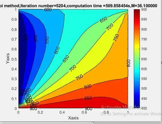
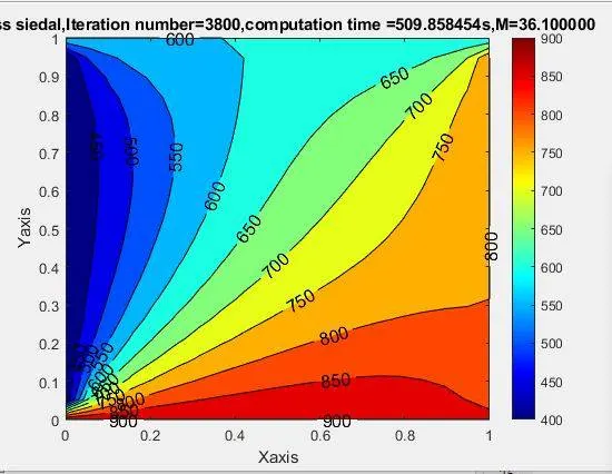
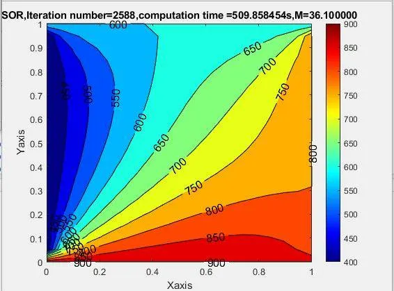
Plottings:

For jacobi method:

For gauss seidal method:

For SOR method:

Result:

As we can see from the results of explicit and implicit methods,explicit method is much faster than the implicit method.

Computational time for explicit method is 0.171388s.

Fastest method in implicit is the sor with 2588 iterations.

But from the explicit and implicit method,implicit is much accurate as it uses various iterative solvers to converge the solution and above it uses all values from the entire domain.