Week 5 - Genetic Algorithm
Aim
1.Understand the concept of Optimization and Genetic Algorithm.
2.Stalagmite function.
Explanation of main terminology
1.Optimization :- process of selecting or finding out values from a given set of values inorder to get dezired output.
2.Population space :- total number of set of values provided in 2D array is called population space.
3.Population size :- Certain values choosen from population space .
Equations used
Range of y = 0 to 0.6
Syntax for GA
X = ga(fun , nvariable , A , B , Aeq , Beq , lb , up , nonl con , options)
here
fun = Function used.
nvariable = number of variables.
A = linear inequality constraints (real matrix)
B = linear inequality constraints (real vector)
Aeq = linear equality constraints (real matrix)
Beq = linear equality constraints (real vector)
lb =lower limits
up =lower limits
nonl con =non linear constraints
options = optimization options
Function code used
function[f]= stalagmite_fun(input)


f1 = (sin(((5.1*pi).*input(1))+0.5)).^6;

f2= (sin(((5.1*pi).*input(2))+0.5)).^6;

f3= exp((-4*log(2).*(((input(1)-0.0667).^2)./0.64)));

f4= exp((-4*log(2).*(((input(2)-0.0667).^2)./0.64)));

f = -(f1.*f2.*f3.*f4);
end
Case no. 1
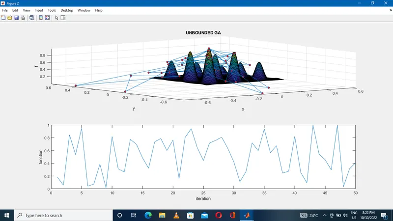
Unbounded GA study - In this case lower and upper bounds are not defined or we can say that no any limits are provided within the axis.
Code
clear all
close all
clc


x = linspace(0,0.6,150);         %creating 1d array for x
y = linspace(0,0.6,150);         %creating 1d array for x

[xx,yy] = meshgrid(x,y);         %conversion of 1d array into 2d array
num_cases = 50;                  % define no. itration

%initialize nested for loop
for i = 1:length(xx)             % initialize indexing for xx

   for j= 1:length(yy)           % initialize indexing for xx
input(1) = xx(i,j);              %define inputs
input(2) = yy(i,j);              %define inputs

f(i,j) = stalagmite_fun(input);  %computing 'f' by calling function 'stalgmite_fun'
   end
end
figure(1)                        %creating separate figure
surf(xx,yy,f)
xlabel('xx')                     %labelinf for x axis
ylabel('yy')                     %labelinf for y axis
zlabel('f')                      %labelinf for z axis
shading interp                   % meshing segment line and face of

%case no.1
%unbounded
tic
for i = 1:num_cases;              % generating for loop
    [inputs,fopt(i)] = ga(@stalagmite_fun,2);  %computing optimam value of f ,x and y
    xopt(i) = inputs(1);          %define xopt
    yopt(i) = inputs(2);          %define xopt

end
time_study = toc
figure(2)
subplot(2,1,1)                    %breaking of figure into 2x1 size

surfc(x,y,-f)                     %creating 3d surface plot
hold on
xlabel('x')              %labelinf for x axis
ylabel('y')              %labelinf for y axis
zlabel('f')              %labelinf for z axis
%ploting of xopt,yopt,fopt in 3d by using plot3
plot3(xopt,yopt,-fopt,'Marker',"o",'MarkerSize',5,'MarkerFaceColor','r')

 title('UNBOUNDED GA')            %give title to plot


subplot(2,1,2)

plot(-fopt)                      %ploting -fopt
xlabel('iteration')              %labelinf for x axis
ylabel('function')               %labelinf for x axis
code outputs
Case no. 2
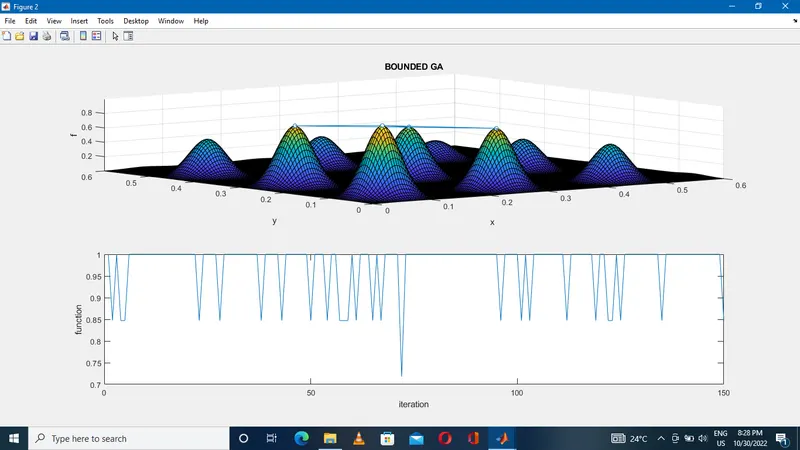
Bounded GA study - In this case upper and lower limits are provided .
limits are defined as blow
For x lower limit is 0 and upper limit is 0.4
For y lower is 0 and upper is 0.4
Code
clear all
close all
clc

x = linspace(0,0.6,150);                %creating 1d array for x
y = linspace(0,0.6,150);                %creating 1d array for y


[xx,yy] = meshgrid(x,y);                %conversion of 1d array into 2d array
num_cases = 150;                        % define no. itration


%initialize nested for loop
for i = 1:length(xx)                     % initialize indexing for xx

   for j= 1:length(yy)                   % initialize indexing for yy
input(1) = xx(i,j);                      % define inputes
input(2) = yy(i,j);                      % define inputes

f(i,j) = stalagmite_fun(input);      %computing 'f' by calling function 'stalgmite_fun'
   end
end
figure(1)
surf(xx,yy,f)
shading interp


%case no.2
%bounded
tic
for i = 1:num_cases;      %creating separate figure%creating separate figure

     %computing optimam value of f ,x and y
    [inputs,fopt(i)] =  ga(@stalagmite_fun,2,[],[],[],[],[0,0],[0.4,0.4]);
    xopt(i) = inputs(1);
    yopt(i) = inputs(2);

end
time_study = toc
figure(2)
subplot(2,1,1)

surfc(x,y,-f)

xlabel('x')              %labelinf for x axis
ylabel('y')              %labelinf for y axis
zlabel('f')              %labelinf for z axis
hold on

%ploting of xopt,yopt,fopt in 3d by using plot3
plot3(xopt,yopt,-fopt,'Marker',"o",'MarkerSize',5,'MarkerFaceColor','auto')

title('BOUNDED GA')

subplot(2,1,2)

plot(-fopt)
xlabel('iteration')
ylabel('function')
code output
Case no. 3
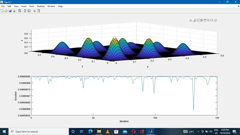
Bounded GA study with population size - In this case population size also provide with lower and upper limits.
here we take population size 250
code
clear all
close all
clc

x = linspace(0,0.6,100);              %creating 1d array for x
y = linspace(0,0.6,100);              %creating 1d array for x

[xx,yy] = meshgrid(x,y);              %conversion 1d aaray into 2d
num_cases = 150;                      %define iteration number

%initialize nested for loop
for i = 1:length(xx)                 % indexing for xx

   for j= 1:length(yy)               %indexing for yy
input(1) = xx(i,j);                  %define inputs
input(2) = yy(i,j);                  %define inputs

f(i,j) = stalagmite_fun(input);      %computing 'f' by calling function 'stalgmite_fun'
    end
 end
 figure(1)                          % create seperate figure
 surf(xx,yy,f)
 shading interp


%case no.3
%bounded ga with population size
options = optimoptions('ga');
options = optimoptions(options,'PopulationSize',250);     %defining population size


%tic
for i = 1:num_cases;        %initialize for loop

 %computing optimam value of f ,x and y
    [inputs,fopt(i)] =  ga(@stalagmite_fun,2,[],[],[],[],[0,0],[0.4,0.4],[],[],options);
    xopt(i) = inputs(1);
    yopt(i) = inputs(2);

end
time_study = toc
 figure(2)
 subplot(2,1,1)

surfc(x,y,-f)

xlabel('x')              %labelinf for x axis
ylabel('y')              %labelinf for y axis
zlabel('f')              %labelinf for z axis
  hold on
  plot3(xopt,yopt,-fopt,'Marker',"o",'MarkerSize',10,'MarkerFaceColor','auto')
%
% title('BOUNDED GA WITH POPULATION SIZE')
%
 subplot(2,1,2)

plot(-fopt)
xlabel('iteration')
ylabel('function')
Code output
Conclusion
in caes 1 (unbounded GA) we does not have limits for x and y axis so we get values of function irrespective of given rang hance there is chances to get inaccurate solution.
but in case 2(bounded GA) we have provided the limits for x and y axis thats why get better and accurate solution .
since by provided limits for axis we still not get optimum solution so in case 3 we introduce population size also hance we get our optimum solution