Week 5 - Genetic Algorithm

stalagmite function :-

function [f] = stalagmite(input_vector)
x = input_vector(1);
y = input_vector(2);

f1x = (sin((5.1*pi*x)+0.5))^6;
f1y = (sin((5.1*pi*y)+0.5))^6;
f2x = exp(-4*log(2)*((x-0.0667)^2)/0.64);
f2y = exp(-4*log(2)*((y-0.0667)^2)/0.64);

f = -(f1x*f1y*f2x*f2y);
end

Main Code :-

clear all
close all
clc

%Definie our search space
x = linspace(0,0.5,150);         %x array
y = linspace(0,0.5,150);         %y array
n = 50;                          %number of cases

%Creating a 2D mesh
[xx,yy] = meshgrid(x,y);

%creating a loop for Evaluating a stalagmite function
for i = 1:length(xx)
    for j = 1:length(yy)
        input_vector(1)=xx(i,j);
        input_vector(2)=yy(i,j);
        f(i,j) = stalagmite(input_vector);
    end
end

%Study 1 : Statistical Behaviour
tic
for i = 1:n
    [inputs,fopt(i)] = ga(@stalagmite,2);
    xopt(i) = inputs(1);
    yopt(i) = inputs(2);
end

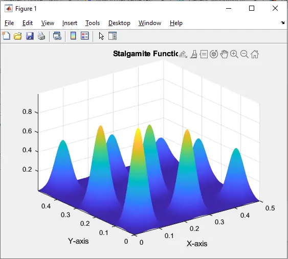
figure(1)
surfc(xx,yy,-f)
shading interp
xlabel('X-axis')
ylabel('Y-axis')
title('Stalgamite Function')

study1_time = toc
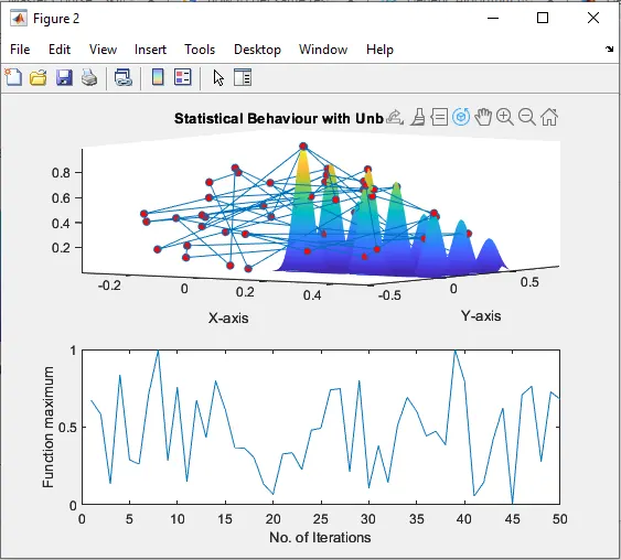
figure(2)
subplot(2,1,1)
hold on
surfc(xx,yy,-f)
shading interp
xlabel('X-axis')
ylabel('Y-axis')
title('Statistical Behaviour with Unbound inputs')
plot3(xopt,yopt,-fopt,'marker','o','markersize',5,'markerfacecolor','r')
subplot(2,1,2)
plot(-fopt)
xlabel('No. of Iterations')
ylabel('Function maximum')

%Study2 : Statistical behaviour with upper and lower bounds
tic
for i = 1:n
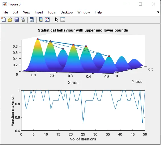
    [inputs,fopt(i)] = ga(@stalagmite,2,[],[],[],[],[0;0],[1;1]);
    xopt(i) = inputs(1);
    yopt(i) = inputs(2);
end
study2_time = toc

figure(3)
subplot(2,1,1)
hold on
surfc(xx,yy,-f)
shading interp
xlabel('X-axis')
ylabel('Y-axis')
title('Statistical behaviour with upper and lower bounds')
plot3(xopt,yopt,-fopt,'marker','o','markersize',5,'markerfacecolor','r')
subplot(2,1,2)
plot(-fopt)
xlabel('No. of Iterations')
ylabel('Function maximum')

%Study3 : Statistical Behaviour with increasing iterations of GA
options = optimoptions('ga');
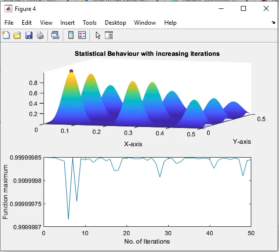
options = optimoptions(options,'PopulationSize',300);

tic
for i = 1:n
    [inputs,fopt(i)] = ga(@stalagmite,2,[],[],[],[],[0;0],[1;1],[],[],options);
    xopt(i) = inputs(1);
    yopt(i) = inputs(2);
end
study3_time = toc

figure(4)
subplot(2,1,1)
hold on
surfc(xx,yy,-f) % 3d plot 
shading interp  % this command used to make plot smooth, it hide shading from plot
xlabel('X-axis')
ylabel('Y-axis')
title('Statistical Behaviour with increasing iterations')
plot3(xopt,yopt,-fopt,'marker','o','markersize',5,'markerfacecolor','r')
subplot(2,1,2)
plot(-fopt)
xlabel('No. of Iterations')
ylabel('Function maximum')

Output :-

GA Syntax :-

• x = ga(fun,nvar,A,b,Aeq,beq,lb,ub,nonlcon,options)
• fun = objective function
• nvar = number of variable
• A,b = Linear inequality constrained
• Aeq, beq = Linear equality constrained
• Lb, ub = Lower bound & Upper bound
• Nonlcon = Nonlinear constrained
• Options = Optimization option

A genetic algorithm (GA) is a method for solving both constrained and unconstrained optimization problems based on a natural selection process that mimics biological evolution.

it is udsed to find aglobal maxima .