Project 2 - Rankine cycle Simulator

- Rankine Cycle Simulator

• Calculate the state points of the Rankine Cycle based on given inputs.
• Plot the corresponding T-S and H-S plots for the given set of inputs.

Input Values:

• Turbine Inlet temperature = 400° C
• Turbine Inlet Pressure = 30 bars
• Turbine Outlet Pressure = 0.05 bars = Condenser Inlet Pressure

Theory :- Ideal Rankine Cycle

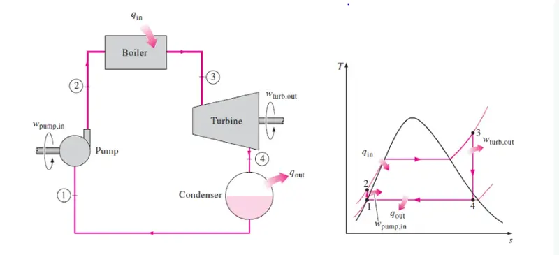
The ideal cycle for vapor power plants is the Rankine cycle. The simple ideal Rankine cycle does not involve any internal irreversibilities and consists of the following four processes:

1-2 Isentropic compression in a pump: Water is pumped from low pressure to high pressure, which is the boiler’s operating pressure. At this stage the fluid is in liquid state so the pump requires little input energy.

2-3 Constant pressure heat addition in a boiler: the high pressure liquid enters a boiler where it is heated at constant pressure by an external heat source to become dry saturated vapor. Steam tables can be used to calculate the input energy.

3-4 Isentropic expansion in a turbine: the dry saturated vapor enters a turbine where it expands isentropically, generating power by rotating the shaft connected to an electric generator. Steam leaves the turbine as a liquid-vapor mixture with high energy levels.

4-1 Constant pressure heat rejection in a condenser: Condensers are heat exchangers that typically use lakes, rivers or the atmosphere where heat is rejected to. At constant pressure, the steam is condensed in a condenser, to become saturated liquid. Then, steam leaves the condenser as saturated liquid and enters the pump, completing the cycle.

- Actual Code :-

% Rankine Cycle Simulator
clear all
close all
clc

% Printing Introduction process of Ideal Rankine Cycle
disp('RANKINE CYCLE SIMULATOR')
disp(' 1-2 is isentropic expansion in the Turbine ')
disp('2-3 is Constant Pressure Heat Rejection by the Condenser ')
disp('3-4 is isentropic Compression in pump')
disp('4-1 is Constant Pressure Heat Addition by the Boiler')

% User Inputs which we have to give while running the code
P1 = input('\n Enter the Pressure at the Turbine Inlet (in bar)='); % 30 bar
T1 = input('\n Enter the Temprature at the Turbine Inlet (in Degree Celcius)='); % 400 C
P2 = input('\n Enter the Pressure at the Turbine Outlet (in bar)='); % 0.05 bar

% State point 1 using a XSteam function , Xsteam function library kept in
% same folder 
H1 = XSteam('h_pt',P1,T1);  %Enthalpy
S1 = XSteam('s_pt',P1,T1);  %Entropy
Hf1 = XSteam('hL_p',P1);    %Enthalpy of saturated liquid
Hg1 = XSteam('hV_p',P1);    %Enthaply of saturated vapour
Ts1 = XSteam('Tsat_p',P1);  %Saturation Temprature
Sf1 = XSteam('sL_p',P1);    %Entropy of saturated liquid
Sg1 = XSteam('sV_p',P1);    %Entropy of saturated vapour

% State point 2
S2 = S1;
Sf2 = XSteam('sL_p',P2);
Sg2 = XSteam('sV_p',P2);
x = (S2-Sf2)/(Sg2-Sf2);     % Dryness fraction
Hf2 = XSteam('hL_p',P2);
Hg2 = XSteam('hV_p',P2);
H2 = Hf2 + x*(Hg2-Hf2);
T2 = XSteam('T_ph',P2,H2);
Ts2 = XSteam('Tsat_p',P2);   

% State point 3
H3 = Hf2;
S3 = Sf2;
T3 = T2;
P3 = P2;

% State point 4
P4 = P1;
S4 = S3;
H4 = XSteam('h_ps',P4,S4);
T4 = XSteam('T_ps',P4,S4);

t = linspace(0,374,500);    % temp space for plotting saturation curves

%Plot T-S Diagram
figure(1)
hold on
% Plot Saturation Curve
for i = 1 : length(t)
   plot(XSteam('sL_T',t(i)),t(i),'.','color','b')
   plot(XSteam('sV_T',t(i)),t(i),'.','color','b')
end
% Plot Cycle
plot([S1 S2],[T1 T2],'linewidth',2,'color','r')
if x>1
    T3 = Ts2;
    plot([S2 Sg2 S3 S4],[T2 Ts2 T3 T4],'linewidth',2,'color','r')
    T2 = Ts2;
else
    plot([S2 S3 S4],[T2 T3 T4],'linewidth',2,'color','r')
end
l = linspace(T1,T2,1000);
for i = 1 : length(l)
    plot(XSteam('s_pT',P1,l(i)),l(i),'.','color','r')
end
plot([Sf1 Sg1],[Ts1 Ts1],'linewidth',2,'color','r')
text(S1+0.05,T1,'1')
text(S1+0.05,T2,'2')
text(S3,T3 -15,'3')
text(S4,T4 +15,'4')
xlabel('Entropy[KJ/Kg-K]')
ylabel('Temprature[K]')
grid on
title('T-S Diagram')

% Plot H-S Diagram
figure(2)
hold on
% Plot Saturation Curve
for i = 1 : length(t)
    plot(XSteam('sL_T',t(i)),XSteam('hL_T',t(i)),'.','color','g')
    plot(XSteam('sV_T',t(i)),XSteam('hV_T',t(i)),'.','color','g')
end
% Plot Cycle with all state points
plot([S1 S2 S3 S4 S1],[H1 H2 H3 H4 H1],'linewidth',2,'color','r')
text(S1+0.05,H1,'1')
text(S1+0.05,H2,'2')
text(S3,H3 -20,'3')
text(S4,H4 +20,'4')
xlabel('Entropy[KJ/Kg-K]')
ylabel('Enthalpy[KJ/Kg]')
grid on
title('H-S Diagram')

% calculations

% Turbine Work
Wt = H1-H2;

% Pump Work
Wp = H4-H3;

% Heat Addition
Qin = H1-H4;

% Heat Rejection
Qout = H2-H3;

% Net Work
Wnet = Wt-Wp;

% Efficiency
Ntherm = (Wnet/Qin)*100;

% Specific steam consumption
SSC = 3600/Wnet;

% Back Work Ratio
BWR = Wp/Wt;

% Print the output Results
disp('Output  Results')

fprintf('At State Point 1:\n')
fprintf('P1 is : %.2f bar \n',P1)
fprintf('T1 is : %.2f Deg Celcius \n',T1)
fprintf('H1 is : %.2f KJ/Kg \n',H1)
fprintf('S1 is : %.2f KJ/Kg-K \n',S1)

fprintf('At State Point 2:\n')
fprintf('P2 is : %.2f bar \n',P2)
fprintf('T2 is : %.2f Deg Celcius \n',T2)
fprintf('H2 is : %.2f KJ/Kg \n',H2)
fprintf('S2 is : %.2f KJ/Kg-K \n',S2)

fprintf('At State Point 3:\n')
fprintf('P3 is : %.2f bar \n',P3)
fprintf('T3 is : %.2f Deg Celcius \n',T3)
fprintf('H3 is : %.2f KJ/Kg \n',H3)
fprintf('S3 is : %.2f KJ/Kg-K \n',S3)

fprintf('At State Point 4: \n')
fprintf('P4 is : %.2f bar \n',P4)
fprintf('T4 is : %.2f Deg Celcius \n',T4)
fprintf('H4 is : %.2f KJ/Kg \n',H4)
fprintf('S4 is : %.2f KJ/Kg-K \n',S4)

fprintf('Wt is : %.2f KJ/Kg \n',Wt)
fprintf('Wp is : %.2f KJ/Kg \n',Wp)
fprintf('Wnet is : %.2f KJ/Kg \n',Wnet)
fprintf('Thermal Efficiency is : %.2f percent \n',Ntherm)
fprintf('S.S.C. is : %.2f Kg/KWh \n',SSC) 
fprintf('Back Work Ratio is : %.3f  \n',BWR)

Output :-

T-S Diagram

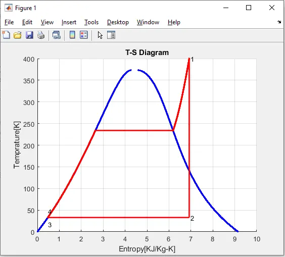
here Blue curve represent the saturation curve and the red color represent the actual rankine cycle with all state points

H-S Digram :-

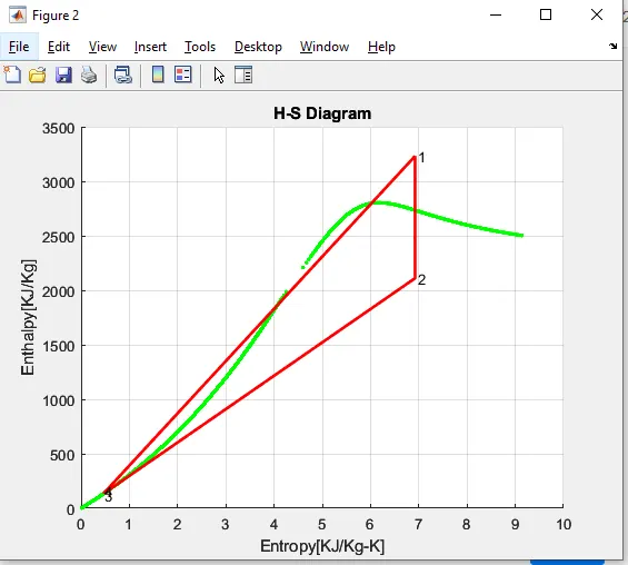
Here green color plot represent the saturation curve and red reresent actual cycle state point

Output Calculation

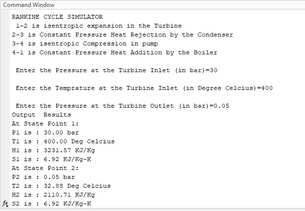
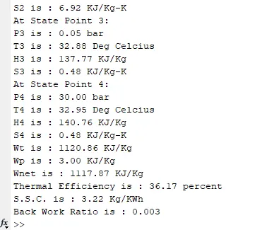
successfuly done the calculation