Week 5 - Genetic Algorithm

GENETIC ALGORITHM: INTRODUCTION

Genetic Algorithm is a method of optimization of an objective function based on the Natural Selection Principle or Survival of the Fittest. It is used to find the minimum or maximum of the objective function through the following steps:

1. Set Initial variables.
2. Define Objective Function and Optimization Goal.
3. Select a family of First Generation of values from the Range of Objective Function. This can follow a certain rule or be random or/and subject to certain constraints.
4. Give a Fitness value for this Generation of DATA. Higher Fitness Value corresponds to a higher probability of getting selected.
5. Randomly Select one or a Set of values for crossover to the next generation. (ex. Roullette Wheel)
6. Mutate the Values. This means introducing changes in the selection criteria will give a better result.
7. Evaluate the Final Result and Repeat from Selection If Needed.

ga() function in MATLAB

The function ga is used to perform genetic algorithm in MATLAB. It is function in the optimization tool kit in MATLAB.

Syntax used in this program is given below, there are more variation in MATLAB HELP.

function f=stalagmite(input_vector)
x=input_vector(1);
y=input_vector(2);

f1x=(sin(5.1.*pi.*x-0.5).^6);
f1y=(sin(5.1.*pi.*y-0.5).^6);
f2x=exp(-4.*log(2).*((x-0.0667).^2)/.64);
f2y=exp(-4.*log(2).*((y-0.0667).^2)/.64);

%modified objective stalagmite function to find maximum 
f=-1.*f1x.*f1y.*f2x.*f2y;
end

• Defining the Search Space. Use linspace cammand to create x and y of length 150 from 0 to 0.6.
• Mesh x and y using Meshgrid command to create Two Dimentional Arrays xx and yy.
• Use one for loop inside another with i=1to length(xx) and j=1to length(yy). Define f(i,j)=Stalagmite([xx(i,j) yy(i,j)]) for plotting the graph.
• Study 1- Unbounded Inputs:
  • Run 50 iterations of ga() for the stalagmite function and store the values in xopt,yopt and fopt.
  • In subplot(2,1,1) the Stalagmite function using surfc function.
  • Use shading interp to get clean surface.
  • plot3 is used to mark the iterations of ga.
  • plot fopt vs no. of iterations in subplot(2,1,2)
  • mark fm which most minimum value of the iteration.
• Study 2- Inputs with Lower and Upper Bound as shown in lecture except the limit is [0,0.6]:
  • Run 50 iterations of ga(with limit as per above syntax) for the stalagmite function and store the values in xopt,yopt and fopt.
  • In subplot(2,1,1) the Stalagmite function using surfc function.
  • Use shading interp to get clean surface.
  • plot3 is used to mark the iterations of ga.
  • plot fopt vs no. of iterations in subplot(2,1,2)
  • mark fm which most minimum value of the iteration.
• Study 3- Inputs with limits and options:
  • Invoke options=optimoptions('ga')
  • In the options 'PopulationSize', 'FunctionTolerance', 'MutationFcn' are selected.
  • 'PopulationSize' - Size of the population. 100 is size selected after trails to get best results in best time.
  • 'FunctionTolerance' - The algorithm stops if the average relative change in the best fitness function value over MaxStallGenerations generations is less than or equal to FunctionTolerance. .0000001 is the assigned value ensures minimum deviation from minimum value of function.
  • 'MutationFcn'-there are several options associated with this function and 'mutationadaptfeasible' is used as it reduced the cycle time.
  • Run 50 iterations of ga() for the stalagmite function and store the values in xopt,yopt and fopt.
  • In subplot(2,1,1) the Stalagmite function using surfc function.
  • Use shading interp to get clean surface.
  • plot3 is used to mark the iterations of ga.
  • plot fopt vs no. of iterations in subplot(2,1,2)

PROGRAM:

close all
clear all
clc

%Defining our search space
x = linspace(0,.6,150);
y = linspace(0,.6,150);
num_cases=50;


%Creating a 2D mesh
[xx yy] = meshgrid(x,y);

%Assigning Function values to f(i,j)
for i=1:length(xx)
    for j=1:length(yy)
        inputvector(1)=xx(i,j);
        inputvector(2)=yy(i,j);
        f(i,j)=stalagmite(inputvector);
    end
end

%Study 1 - Unbounded inputs
tic
fm=0;%Maximum Value
maxima_pos=0;%Maxima Position
for k=1:num_cases
[inputs, fopt(k)] = ga(@stalagmite,2);
xopt(k)=inputs(1);
yopt(k)=inputs(2);
if fm>fopt(k)
    fm=fopt(k);
    maxima_pos=k;
end
end

%plot #1
figure(1)
subplot(2,1,1)
hold on
surfc(xx,yy,f)
title('UNBOUNDED INPUTS')
xlabel('x axis')
ylabel('y axis')
zlabel('Function Value')
shading interp
plot3(xopt,yopt,fopt,'marker','O','MarkerSize',5,'MarkerFaceColor','r')
subplot(2,1,2)
plot(fopt)
hold on
plot3(maxima_pos,fopt(maxima_pos),0,'marker','O','MarkerSize',5,'MarkerFaceColor','r')
xlabel('No. of Iterations')
ylabel('Function Minimum')

Study_of_time_1 = toc

%Study 2 - With Limits 0<x<0.6 and 0<y<0.6
tic
fm=0;%Maximum Value
maxima_pos=0;%Maxima Position
for k=1:num_cases
[inputs, fopt(k)] = ga(@stalagmite,2,[],[],[],[],[0;0],[0.6;0.6]);
xopt(k)=inputs(1);
yopt(k)=inputs(2);
if fm>fopt(k)
    fm=fopt(k);
    maxima_pos=k;
end
end

%plot #2
figure(2)
subplot(2,1,1)
hold on
surfc(xx,yy,f)
title('BOUNDED INPUTS')
xlabel('x axis')
ylabel('y axis')
zlabel('Function Value')
shading interp
plot3(xopt,yopt,fopt,'marker','O','MarkerSize',5,'MarkerFaceColor','r')
subplot(2,1,2)
plot(fopt)
hold on
plot3(maxima_pos,fopt(maxima_pos),0,'marker','O','MarkerSize',5,'MarkerFaceColor','r')
xlabel('No. of Iterations')
ylabel('Function Minimum')

Study_of_time_2 = toc

%Study 3 - With Limits and options
options=optimoptions('ga')
options=optimoptions(options,'PopulationSize',100,'FunctionTolerance',.0000001,'MutationFcn','mutationadaptfeasible')
tic
fm=0;%Maximum Value
maxima_pos=0;%Maxima Position
for k=1:num_cases
[inputs, fopt(k)] = ga(@stalagmite,2,[],[],[],[],[0;0],[0.6;0.6],[],options);
xopt(k)=inputs(1);
yopt(k)=inputs(2);
if fm>fopt(k)
    fm=fopt(k);
    maxima_pos=k;
end
end

%plot #3
figure(3)
subplot(2,1,1)
hold on
surfc(xx,yy,f)
title('BOUNDED INPUTS with OPTIONS')
xlabel('x axis')
ylabel('y axis')
zlabel('Function Value')
shading interp
plot3(xopt,yopt,fopt,'marker','O','MarkerSize',5,'MarkerFaceColor','r')
subplot(2,1,2)
plot(fopt)
hold on
plot3(maxima_pos,fopt(maxima_pos),0,'marker','O','MarkerSize',5,'MarkerFaceColor','r')
xlabel('No. of Iterations')
ylabel('Function Minimum')

Study_of_time_3= toc
Study_of_time_2
Study_of_time_1

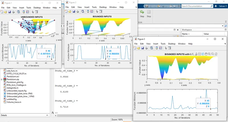
FINAL RESULTING PLOT:

NOTE:-FIGURE 3 minimum varies by a low margin