Week 3 - Solving second order ODEs

EXPLANATION:

1. BASIC PRINCICLE AND FORMULA:
   • The Basic 2nd Order Ordinary Differential Equation for the motion of a pendulum is                   
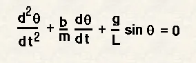
   • This is simplified to Equation 1 and 2 respectively, Theta1 = d(theta)/dt and (d(theta1)/dt)+(b/m)*theta1+(g/L)*sin(Theta)=0.
   • Where, b-damping, m-mass, g-acceleration of gravity, L-length of pendulum, theta-angle of pendulum.
2. FLOW OF THE PROGRAM
   • Define the Inputs b,m,g and L.
   • Set limits for theta_0 in column array.
   • Define t_span for 10 secs using linspace command.
   • Define matrix [t, results] equal to Call function ode45((@(t, theta) ode_func(t,theta,b,g,L,m), t_span, theta_0).
   • @(t, theta) defines t and theta as independent and dependent variables respectively.
   • ode_func relates a column matrix with dtheta/dt and dtheta1/dt according to given formula.
   • ode45 solves the 2 differential equations according to the given formula in ode_func and returns the corresponding theta and theta1 values for every t_span value.
   • Plot1:-plots theta and theta1 values from [results] against time.
   • Animation:-for loop with range from 1 to length of [t_span]
   • define x=L*sin(theta) and y=x=L*cos(theta).
   • plot line at (x -y), then use hold on and plot the letter 'O' with a linewidth of 6(makes the bob), then pause(t_span(i+1)-t_span(i)) and finally hold off. end loop.
3. FUNCTIONS
   • Saves the two first order differential equations and returns the final values to ode45.
   • dtheta1/dt = theta2;

     dtheta2/dt = -(b/m)*theta2 - (g/L)*sin(theta1); Returns[dtheta/dt dtheta1/dt]
4. ERRORS
   • had to use hold on after line plot and hold off at the end of loop to get the animation properly. 
5. OUTPUT
   • outputs 500 values of [theta theta1] in command window.
   • Figure(1) plot of theta and theta1 vs t.
   • animation of pendulum. video link https://youtu.be/aPoWHLksHN4

CODE:

clear all
close all
clc

%defining the INPUTS
b=.05;
g=9.81;
m=.1;
L=1;
ct=1;

%Setting the limits of theta
theta_0 = [0;5];

%defining the time Span
t_span = linspace(0,10,500);

%Solving the ODE using ODE45 function
[t, results] = ode45(@(t, theta) ode_func(t,theta,b,g,L,m), t_span, theta_0);

%plot
figure(1)
plot(t,results(:,1))
hold on
plot(t, results(:,2))
ylabel('Plot')
xlabel('Time')
legend('theta','theta1')
%Animation of pendulum
for i=1:length(t_span)-1
    x = L*sin(results(i,1));
    y = L*cos(results(i,1));
    figure(2)
    plot([0 x],[0 -y],'LineWidth',3)
    hold on
    plot(x,-y,'O','LineWidth',6)
    axis([-1 1, -1.5 0])
    pause(t_span(i+1)-t_span(i))
    hold off
    M(ct) = getframe(gcf);
    ct=ct+1;  
end

movie(M)
videofile = VideoWriter('Pendulum.avi','uncompressed AVI');
open(videofile)
writeVideo(videofile,M)
close(videofile)

FUNCTION:

function dtheta_dt = ode_func(t,theta,b,g,L,m)

theta1 = theta(1);
theta2 = theta(2);
dtheta1_dt = theta2;
dtheta2_dt = -(b/m)*theta2 - (g/L)*sin(theta1);
dtheta_dt = [dtheta1_dt; dtheta2_dt]

end