Challenge

Week 5 - Genetic Algorithm

HHarshal Dhandrut26 Dec 2023

Genetic Algorithm

A Genetic Algorithm is a search heuristic inspired by the process of natural selection and genetics. It is commonly used to find approximate solutions to optimization and search problems. The algorithm operates on a population of potential solutions, encoding them as individuals, and evolves the population over generations.

The ga function in MATLAB is used to perform genetic algorithm optimization. The basic syntax is as follows:

[x, fval] = ga(fun, nvars)

fun: The objective function to be minimized or maximized.

nvars: The number of variables in the optimization problem.

Additional parameters and options can be provided to customize the behavior of the genetic algorithm. For example:

[x, fval] = ga(fun, nvars, A, b, Aeq, beq, lb, ub, nonlcon, options)

A, b: Linear inequality constraints.

Aeq, beq: Linear equality constraints.

lb, ub: Lower and upper bounds for the variables.

nonlcon: Nonlinear constraint function.

options: A structure containing various options for the genetic algorithm.

Matlab code :

clear all

close all

clc

% Define parameters

n = 150; % Number of iterations

x = linspace(0, 0.6, 150);

y = linspace(0, 0.6, 150);

% Creating two-dimensional grid

[xx, yy] = meshgrid(x, y);

% Evaluate the stalagmite function on the grid

tic

for i = 1:length(xx)

for j = 1:length(yy)

input_vector(1) = xx(i, j);

input_vector(2) = yy(i, j);

f(i, j) = stalagmite(input_vector);

end

% Plot the surface plot of the stalagmite function

figure(1)

surfc(xx, yy, f)

shading interp

xlabel('x value');

ylabel('y value');

title('Stalagmite Function Surface Plot');

study_time = toc; % Record the time taken for function evaluation

% Case 1: Unbounded inputs using fminsearch

tic

for i = 1:n

% Use fminsearch to optimize the stalagmite function

[inputs, fopt(i)] = fminsearch(@stalagmite, rand(1, 2));

xopt(i) = inputs(1);

yopt(i) = inputs(2);

end

% Plot the results for unbounded inputs

figure(2)

subplot(2, 1, 1)

hold on

surfc(x, y, -f)

shading interp

plot3(xopt, yopt, -fopt, 'marker', 'o', 'markersize', 5, 'markerfacecolor', 'r')

title('Unbounded Inputs')

subplot(2, 1, 2)

plot(-fopt)

xlabel('no. of iterations');

ylabel('function max');

study_time1 = toc; % Record the time taken for optimization

% Case 2: Bounded inputs using fminsearch

tic

for i = 1:n

% Use fminsearch to optimize the stalagmite function with bounds

inputs = fminsearch(@(x) stalagmite(x), rand(1, 2));

xopt(i) = inputs(1);

yopt(i) = inputs(2);

fopt(i) = stalagmite(inputs);

end

% Plot the results for bounded inputs

figure(3)

subplot(2, 1, 1)

hold on

surfc(x, y, -f)

shading interp

plot3(xopt, yopt, -fopt, 'marker', 'o', 'markersize', 5, 'markerfacecolor', 'r')

title('Bounded Inputs')

subplot(2, 1, 2)

plot(-fopt)

xlabel('no. of iterations');

ylabel('function max');

study_time2 = toc; % Record the time taken for optimization

% Case 3: Bounded inputs with increased population using fmincon

tic

options = optimoptions('fmincon', 'Display', 'off');

for i = 1:n

lb = [0; 0]; % Lower bounds

ub = [0.6; 0.6]; % Upper bounds

% Use fmincon to optimize the stalagmite function with bounds and options

inputs = fmincon(@(x) stalagmite(x), rand(2, 1), [], [], [], [], lb, ub, [], options);

xopt(i) = inputs(1);

yopt(i) = inputs(2);

fopt(i) = stalagmite(inputs);

end

% Plot the results for bounded inputs with increased population

figure(4)

subplot(2, 1, 1)

hold on

surfc(x, y, -f)

shading interp

plot3(xopt, yopt, -fopt, 'marker', 'o', 'markersize', 5, 'markerfacecolor', 'r')

title('Bounded Inputs with Increased Population')

subplot(2, 1, 2)

plot(-fopt)

xlabel('no. of iterations');

ylabel('function max');

study_time3 = toc; % Record the time taken for optimization

Stalagmite function code :

function [f] = stalagmite(input_vector)

f1x = (sin((5.1*pi).*input_vector(1)+0.5)).^6;

f1y = (sin((5.1*pi).*input_vector(2)+0.5)).^6;

f2x = exp((((input_vector(1)-0.0667).^2)/0.64).*(-4*log(2)));

f2y = exp((((input_vector(2)-0.0667).^2)/0.64).*(-4*log(2)));

f1=f1x*f1y*f2x*f2y;

f=-f1;

end

Plots and observations :

Figure 1: Stalagmite Function Surface Plot

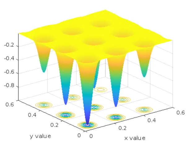
This figure represents the surface plot of the stalagmite function over the given two-dimensional grid.
The surface plot gives a visual understanding of the function's behavior in the specified input space.

Figure 2: Unbounded Inputs Study

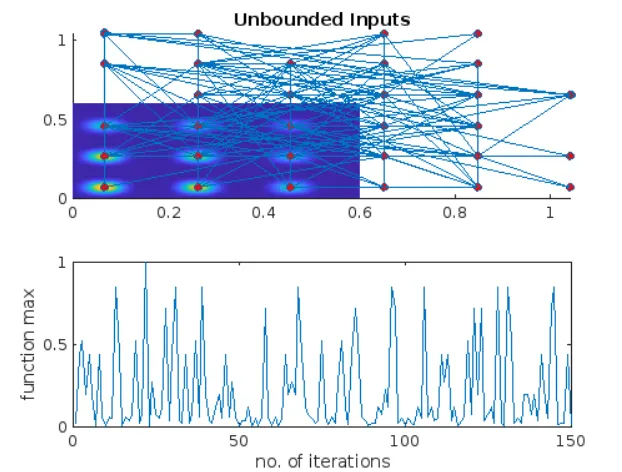
This figure depicts the results of the genetic algorithm optimization for unbounded inputs.
The surface plot shows the original function, and the red markers represent the optimal points found by the genetic algorithm.
The lower subplot illustrates the evolution of the maximum function value over iterations.

Figure 3: Bounded Inputs Study

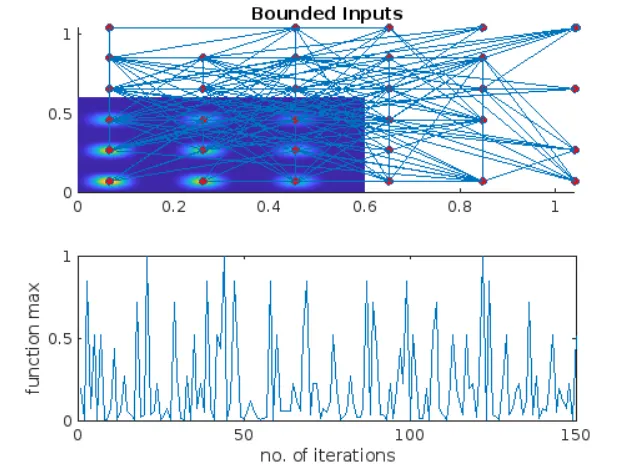
This figure shows the results of the genetic algorithm optimization for bounded inputs.
Similar to Figure 2, the surface plot displays the original function, and the red markers indicate optimal points within the specified bounds.
The lower subplot depicts the convergence of the maximum function value over iterations.

Figure 4: Bounded Inputs with Increased Population Study

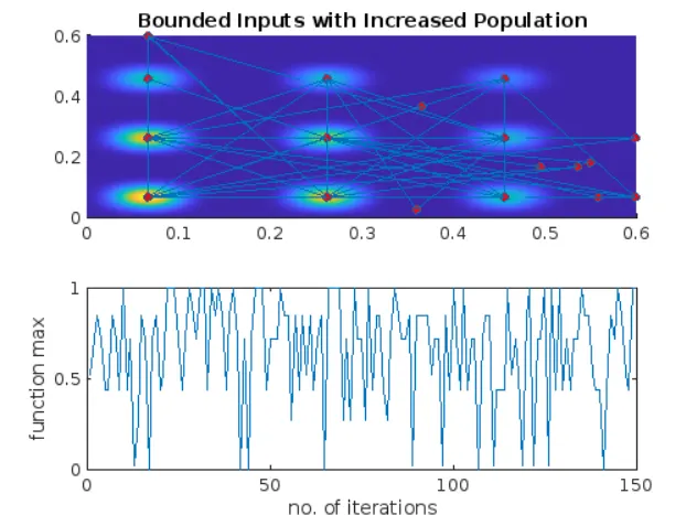
This figure represents the outcomes of the genetic algorithm optimization for bounded inputs with an increased population size.
The surface plot visualizes the original function, and the red markers highlight optimal points found by the genetic algorithm.
The lower subplot shows the progression of the maximum function value with a larger population.

Observations:

In both studies with bounded inputs (Figure 3 and Figure 4), the genetic algorithm successfully finds optimal solutions within the specified bounds.
The use of an increased population in Figure 4 appears to contribute to faster convergence and potentially better solutions.
The convergence behavior and speed can be influenced by various factors, including the choice of optimization algorithm, population size and other algorithm-specific parameters.
Comparing the results of different studies can provide insights into the trade-offs between solution quality, convergence speed, and computational cost.

Week 5 - Genetic Algorithm

Ship work like this
in your own course.

Talk to a career counsellor

Ship work like thisin your own course.

Talk to a career counsellor

Ship work like this
in your own course.