Week 5 - Genetic Algorithm

The concept of Genetic Algorithm

A genetic algorithm is a natural process that is used for the selection of the fittest individuals. The main use of the genetic algorithm is for reproduction to produce offspring of the next generation, this process of selecting and reproducing the fittest individual is inspired by Charles Darwin’s and named it the "Theory of evolution".

Syntax for GA algorithm

The syntax used in this program are as follows: -

x = ga(fun,nvars)-finds a local unconstrained minimum, x, to the objective function, fun. nvars is the dimension (number of design variables) of fun, where, fun- objective function and nvars-number of variables.

x = ga(fun,nvars,A,b,Aeq,beq,lb,ub)- defines a set of lower and upper bounds on the design variables, x, so that a solution is found in the range lb ≤ x ≤ ub. When there is no linear inequalities we set Aeq and Beq as null vector.

x = ga(fun,nvars,A,b,[],[],lb,ub,nonlcon,IntCon) or x = ga(fun,nvars,A,b,Aeq,beq,lb,ub,nonlcon,intcon,options) requires that the variables listed in IntCon take integer values.

Where, A and b are A=[] and b=[] if no linear inequalities.

lb and ub are lower bound and upper bound. Lower bounds, and upper bound specified as a real vector or array of doubles.

nonlcon is a function that accepts a vector or array.

Intcon- integer variable vectors of positive integers.

options- Optimization options, specified as the output of optimoptions or a structure it helps in constraint tolerance by increasing the population size.

Function Code:

function [f] = stalagmite(input_vector)
f1x = (sin((5.1*pi).*input_vector(1)+0.5)).^6;
f1y = (sin((5.1*pi).*input_vector(2)+0.5)).^6;

f2x = exp((((input_vector(1)-0.0667).^2)/0.64).*(-4*log(2)));
f2y = exp((((input_vector(2)-0.0667).^2)/0.64).*(-4*log(2)));
f1=f1x*f1y*f2x*f2y;
f=-f1;
end

MAIN PROGRAM:

clear all %delete all variables 
close all %delete all plots 
clc %clea command window 

%Creating the search space to be optimized
%one dimensional
n=100;
x = linspace(0,0.6,100);
y = linspace(0,0.6,100);

%Creating two dimensional grid
[xx, yy] = meshgrid(x,y);
tic

%Evaluating the stalagmite function
for i = 1:length(xx)
    for j = 1:length(yy)
        input_vector(1)= xx(i,j);
        input_vector(2)= yy(i,j);
        f(i,j) = stalagmite(input_vector);
    end
end

figure(1)
surfc(xx, yy, f)
shading interp
xlabel('x value');
ylabel('y value');

study_time=toc;


%case 1 (unbounded inputs)
tic
for i = 1:n
    [inputs,fopt(i)]= ga(@stalagmite, 2);
    xopt(i)=inputs(1);
    yopt(i)=inputs(2);
end

figure(2)
subplot(2,1,1)
hold on
surfc (x,y,-f)
shading interp
plot3(xopt,yopt,-fopt,'marker','*','markersize',3,'markerfacecolor','r')
title('Unbounded Inputs')
subplot(2,1,2)
plot(-fopt)
xlabel('Number of iterations');
ylabel('Function max');

study_time1=toc;


% second case (bounded inputs)
tic
for i = 1:n
    [inputs,fopt(i)]= ga(@stalagmite, 2,[],[],[],[],[0;0],[0.6;0.6]);
    xopt(i)=inputs(1);
    yopt(i)=inputs(2);
end

figure(3)
subplot(2,1,1)
hold on
surfc (x,y,-f)
shading interp
plot3(xopt,yopt,-fopt,'marker','*','markersize',3,'markerfacecolor','r')
title('Bounded Inputs')
subplot(2,1,2)
plot(-fopt)
xlabel('Number of iterations');
ylabel('Function max');

study_time2=toc;


% third case (bounded inputs with increased population)
tic
options=optimoptions('ga');
options=optimoptions(options,'PopulationSize',400);

for i = 1:n
    [inputs,fopt(i)]= ga(@stalagmite,2,[],[],[],[],[0;0],[1;1],[],[],options);
    xopt(i)=inputs(1);
    yopt(i)=inputs(2);
end

figure(4)
subplot(2,1,1)
hold on
surfc (x,y,-f)
shading interp
plot3(xopt,yopt,-fopt,'marker','*','markersize',3,'markerfacecolor','r')
title('Bounded inputs with increases population')
subplot(2,1,2)
plot(-fopt)
xlabel('Number of iterations');
ylabel('Function max');

study_time3=toc;

Stepwise explanation of the program

The linspace command is used to define search space, and meshgrid command is used to create the 2d array.

Stalagmite function is created using a sub program and result is stored in f variable.

The 3d representation of stalagmite function is presented by plotting figure 1.

Case study 1 – Statistical behaviour (unbounded)

'ga' solver is iterated for 100 times, and no limits are provided for this case.

'ga' solver returns two outputs, one is the minimum function value which is stored in 'fopt(i)' and other is the coordinates of the minimum value which are stored in 'xopt' and 'yopt'. This loop is run for 100 times and results are plotted using plot command.

Two sub plot is created in figure 2, one is showing the 3d representation of stalagmite with optimization results and other is showing the function value.

'Plot3' command is used to plot a set of coordinates connected by line segments.

'tic' and 'toc' command is used for monitoring the time taken to complete the iterations.

There is no upper and lower limit provided, hence algorithm is searching outside the search space i.e. unbounded

Case study 2 – bounded inputs

In case 2 'ga' solver search space is narrow down bysetting upper and lower limits. This narrows down the search space and it becomes easier for the solver to find global minima.

4 null vectors are passed in the solver syntax because there is no linear inequality involved in the stalagmite function.

Results are plotted in figure 3 by running the loop for 100 times.

Case study 3 – bounded inputs with increased population size

In the case 3 with the increased population size the 'ga' solver is run with the bounded inputs.

Population size specifies how many individuals are there in each generation. With a large population size, the genetic algorithm searches the solution space more thoroughly, thereby reducing the chance that the algorithm returns a local minimum that is not a global minimum. However, a large population size also causes the algorithm to run more slowly.

Optimoptions command is used to create optimization options.

options= optimoptions(SolverName) returns a set of default options for the SolverName

Results and discussion

1) Plot for stalagmite function

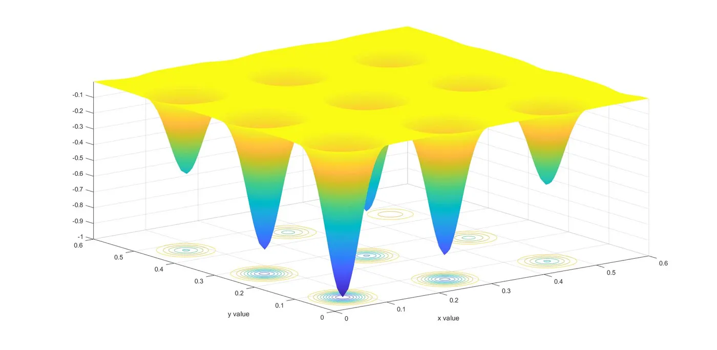
The above plot shows the 3D representation of stalagmite function. A function named stalagmite has been created to evaluate the mathematical expression and store the result in the form of an array. 3D surface plot is created using surfc(X,Y,Z) with a contour plot underneath.

2) Plot for unbounded inputs

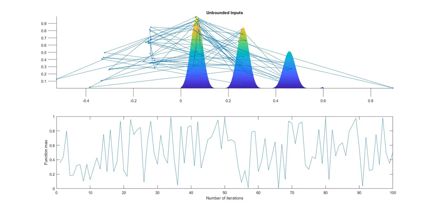
As from the above plot it can be observed that 'ga' solver is unable to calculate the global maxima with the unbounded inputs. further optimization is needed due to random sampling the maximum value ranges between 0.1 to 1.

3) Plot for bounded inputs

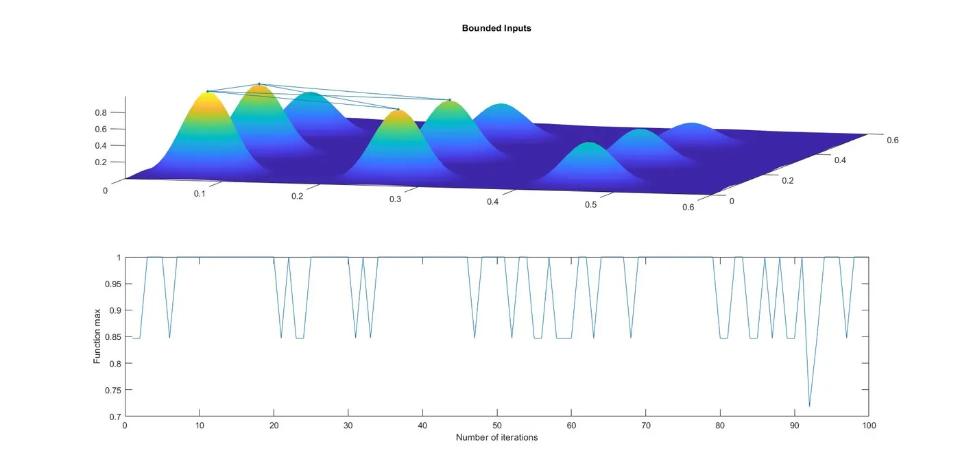
The above plot shows that using 'the bounded inputs' gives more clear result than the previous one. Here the maximum value ranges between 0.7 to 1. But still optimization is needed.

4) Plot for bounded inputs with increased population size

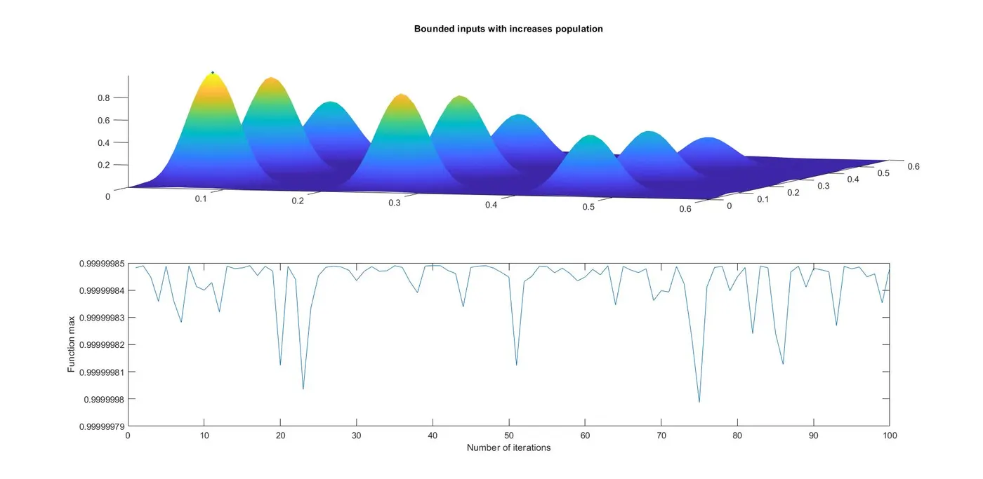
With the increased population size we get the most accurate result.

Conclusions

The ga solver is an inbuilt algorithm in matlab for optimization problem.

Using the solver with bounded inputs gets more accurate results.