Challenge

Week 5 - Genetic Algorithm

NNikhil Kumar12 Aug 2023

Week 5 - Genetic Algorithm

PROBLEM STATEMENT

Try to understand the concept of genetic algorithm by referring to varius sources before you attend this challenge. Look out for information regarding stalagmite function and ways to optimise it.

Write a code in MATLAB to optimise the stalagmite function and find the global maxima of the function.
Clearly expalin the concept of genetic algorithm in your own words and also explain the syntax for ga in MATLAB in your report.
Make sure that your code gives the same output, even if it is made to run several times.
Plot graphs for all 3 studies and for F maximum vs no. of iterations. Title and axes labels are a must, legends could be shown if necessary.

SOLUTION WITH THE REPORT

The concept of Genetic Algorithm

A genetic algorithm is a natural technique for selecting the most suited people. The genetic algorithm is mostly used for reproduction in order to generate children for the following generation; this process of selecting and reproducing the fittest person was inspired by Charles Darwin, who termed it the "Theory of Evolution."

Natural selection begins with the selection of the fittest individuals in a group. They have kids who inherit the qualities of their parents and are passed on to the next generation. If parents are more fit, their children will be fitter than their parents and have a greater chance of survival. This procedure is repeated until a generation of the fittest individuals is discovered.

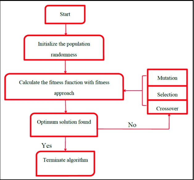
Five phases are considered in a genetic algorithm. They are

Initial population
Fitness function
Selection
Crossover
Mutation

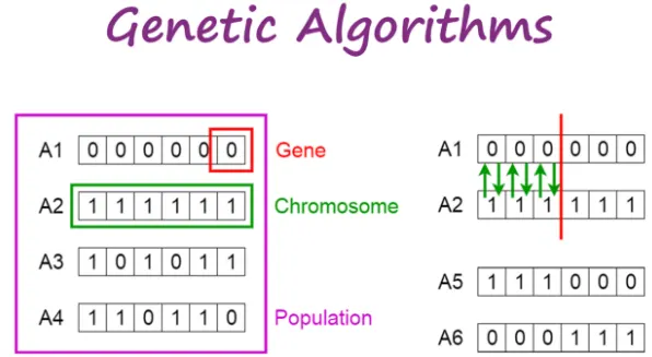
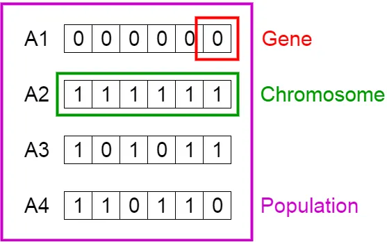
Initial Population- the process begins with a set of individuals which is called a Population. An individual is characterized by a set of parameters (variables) known as Genes. Genes are joined into a string to form a chromosome (solution).

Fitness function - To determine the fitness function we are comparing how fittest an individual is, basically we are comparing the individuals with one another. It gives a fitness score to each individual and based on the fitness score the individual will be selected for reproduction. To perform the optimization in GAs we need to optimize the stalagmite function to find its minima. these have two inputs (x,y).

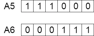
Selection - The idea of the selection phase is to select the fittest individuals and let them pass their genes to the next generation. Here, two pairs of individuals are selected according to their fitness score, higher will be the fitness the more chance is for the selection for reproduction.

Cross over - cross over is a process of taking two-parents' solutions and producing a child from them. For each pair of parents to be mated, a crossover point is chosen at random from within the genes.

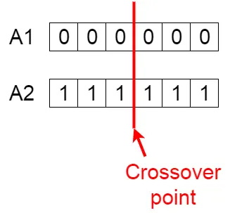
Offspring are created by exchanging the genes of parents among themselves until the crossover point is reached.

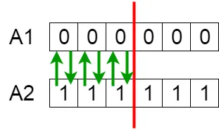
now the new offsprings are added to the population.

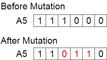
Mutation- Mutation is used to carry out the genetic diversity from one generation of the population of chromosomes to the next generation. This mutation process is too important to perform because if it is not performed then the chromosomes will be too similar to each other. The mutation occurs to maintain diversity within the population and prevent premature convergence and results in local minima.

Advantages of Genetic Algorithms in MATLAB:

Finds Hard Solutions: Genetic Algorithms are good at solving tough problems with many possible solutions.
Works for Different Problems: They can help with many types of problems in different fields.
No Math Tricks Needed: GAs work even when the math is tricky or not clear.
Saves Time with Many Steps: They can do lots of calculations at the same time, which speeds things up.
Easy to Understand: They're based on how nature evolves, so they're easy to grasp.

Limitations of Genetic Algorithms in MATLAB:

Takes a Lot of Computer Work: They need a lot of computer power, especially for complex problems.
Can Be Slow to Finish: They might take a while to find answers, especially for big problems.
Needs Right Settings: You have to set some numbers just right, or they won't work well.
Can Get Lost: Sometimes they focus too much or too little, which can be a problem.
Might Not Get Best Answer: They don't always find the best solution, just a good one.
Doesn't Like Noise: Noise or sudden changes can confuse them.
No Guarantee for Best Answer: They might not find the very best solution.

Syntax For GA Algrorithm

Syntax 1:

x = ga(fun, nvars)

This syntax finds a local unconstrained minimum of the objective function fun, with nvars design variables. The output x is the solution vector that represents the values of the design variables that minimize the objective function.

Syntax 2:

x = ga(fun, nvars, A, b, Aeq, beq, lb, ub)

This syntax finds a solution within bounds for the design variables, while considering linear inequalities and equalities. Here's what each parameter means:

fun: The objective function to minimize.
nvars: The number of design variables.
A: Coefficients for linear inequalities (if any).
b: Right-hand side values for linear inequalities.
Aeq: Coefficients for linear equalities (if any).
beq: Right-hand side values for linear equalities.
lb: Lower bounds for each design variable.
ub: Upper bounds for each design variable.

Syntax 3:

x = ga(fun, nvars, A, b, [], [], lb, ub, nonlcon, IntCon)

x = ga(fun, nvars, A, b, Aeq, beq, lb, ub, nonlcon, IntCon, options)

This syntax adds support for nonlinear constraints and integer variables. Here's what the additional parameters mean:

nonlcon: A function that represents nonlinear constraints. It takes a vector or array of variables and returns constraint values.
IntCon: A vector of indices that specifies which design variables must take integer values.
options: An optional argument for optimization options. It allows you to customize how the genetic algorithm behaves.

To provide more context, let's explain the parameters further:

A, b, Aeq, beq: These parameters define linear inequalities and equalities. If there are none, use empty matrices ([]).
lb, ub: These are arrays specifying lower and upper bounds for each design variable. These bounds restrict the search space of the genetic algorithm.
nonlcon: If you have nonlinear constraints, you can define a separate function for them. The function should accept the variable vector and return constraint values.
IntCon: If you have variables that must be integers, specify their indices in this vector.
options: This is an optional argument that allows you to customize the behavior of the genetic algorithm. You can set parameters related to population size, constraint tolerance, display options, etc.

The GA algorithm tries to find the best solution within the specified bounds and constraints by evolving a population of potential solutions over generations. The optimization process aims to minimize the given objective function while respecting the constraints.

Stalagmite function

Stalagmite is a type of rock formation that rises from the floor of a cave due to the accumulation of material deposited on the floor from ceiling drippings. Stalagmite function is the mathematical function which generates similar shapes to stalagmites. Stalagmite function is a two-variable function, mathematically it is represented as: -

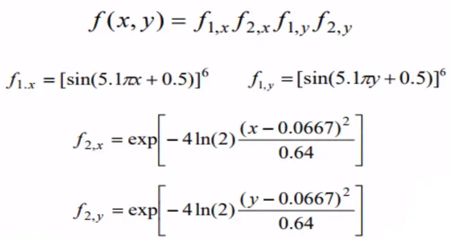
code of the stalagmite function

function [f] = stalagmite(input_vector)
f1x = (sin((5.1*pi).*input_vector(1)+0.5)).^6 ;
f1y =(sin((5.1*pi).*input_vector(2)+0.5)).^6 ;

f2x = exp((((input_vector(1)-0.0667).^2)/0.64).*(-4*log(2)));
f2y = exp((((input_vector(2)-0.0667).^2)/0.64).*(-4*log(2)));

f1 = f1x*f2x*f1y*f2y;
f = -f1;
end

Main Optimisation code

%creating the search space to be optimized
%one dimensional 

clear all
close all
clc

%Inputs
n = 150;
x = linspace(0,0.6,150);
y = linspace(0,0.6,150);

%creating two dimensional grid
[xx , yy] = meshgrid(x,y);

tic

%Evaluating the stalagmite function
for i = 1:length(xx)
    for j = 1:length(yy)
        input_vector(1) = xx(i,j);
        input_vector(2) = yy(i,j);
        f(i,j) = stalagmite(input_vector);
    end
end

figure(1)
surfc(xx , yy , f )
shading interp
xlabel('x-value')
ylabel('y-value')

study_time = toc;

Line by Line explanation of the code

These lines are comments that provide an introduction to the purpose of the code.
clear all clears all variables from the workspace.
close all closes all open figures.
clc clears the command window.
These lines define the parameters of the optimization process and set up the search space.
n is the number of points along each dimension of the grid.
x and y are vectors representing the values of the variables along their respective dimensions. The linspace function generates 150 equally spaced points between 0 and 0.6 for both x and y.
These lines create a two-dimensional grid by using the meshgrid function. This grid covers the entire search space defined by the x and y vectors.
xx and yy are matrices containing the coordinates of each point in the grid.

tic starts a timer to measure the execution time.

These lines implement a nested loop to evaluate the "stalagmite" function for each point in the grid.
The outer loop iterates over i from 1 to the length of xx (number of rows).
The inner loop iterates over j from 1 to the length of yy (number of columns).
input_vector is created for each point with its x and y coordinates.
The "stalagmite" function is called with the input_vector to calculate the function value, which is stored in the matrix f at position (i, j).

These lines create a new figure (Figure 1) for visualization.
surfc is used to create a surface plot of the function values over the xx and yy grid.
shading interp is used to interpolate colors between data points, providing a smoother appearance to the surface.
xlabel and ylabel add labels to the x and y axes.
toc stops the timer and calculates the elapsed time since the tic function was called.

The elapsed time is stored in the variable study_time.This block defines the "stalagmite" function that takes an input_vector as an argument and calculates the function value.

It consists of two main components, f1 and f2, each composed of trigonometric and exponential terms based on the input vector coordinates.
The final function value f is calculated by combining f1 and f2 components and negating the result, as the goal is to minimize the function.

OUTPUT OF THE ABOVE CODES

from the command window

from the workspace

EXPLANATION OF THE OUTPUTS

The 3D depiction of stalagmite function is seen in the plot above.
The mathematical equation will be evaluated by a function called stalagmite, and the result will be saved as an array.
A three-dimensional surface plot with a contour plot beneath has been produced using surfc(X,Y,Z).

CASE STUDY - 1 - STATISTICAL BEHAVIOUR (UNBOUNDED)

CODE FOR THE FOLLOWING:-

clear all
close all
clc

% Inputs
x = linspace(0, 0.6, 50);
y = linspace(0, 0.6, 50);
[X, Y] = meshgrid(x, y);  % Generate a grid of X and Y values
Z = zeros(size(X));

% Preallocate arrays
n = numel(X);
fopt = zeros(1, n);
xopt = zeros(1, n);
yopt = zeros(1, n);

% Case 1 (unbounded inputs)
tic
for i = 1:n
    [inputs, fopt(i)] = ga(@stalagmite, 2);
    xopt(i) = inputs(1);
    yopt(i) = inputs(2);
end

% Calculate Z values using the stalagmite function
for i = 1:n
    Z(i) = -stalagmite([X(i), Y(i)]);
end

figure(2)
subplot(2, 1, 1)
hold on
surfc(X, Y, Z)  % Plot the surface using the grid of values
shading interp
plot3(xopt, yopt, -fopt, 'marker', 'o', 'markersize', 5, 'markerfacecolor', 'r')
title('unbounded inputs')
subplot(2, 1, 2)
plot(-fopt)
xlabel('no. of iterations');
ylabel('function max');

study_time1 = toc;

Function codes will be the same.

line by line explanation of the above codes:-

clear all
close all
clc

These lines clear the workspace, close all open figures, and clear the command window to start with a clean environment.

x = linspace(0, 0.6, 150);
y = linspace(0, 0.6, 150);
[X, Y] = meshgrid(x, y);

These lines create vectors x and y containing 50 equally spaced values between 0 and 0.6. The meshgrid function then generates 2D arrays X and Y which represent a grid of points based on the x and y values. These arrays will be used for plotting the 3D surface and for evaluating the stalagmite function.

Z = zeros(size(X));

This line initializes a 2D array Z with zeros. This array will be used to store the calculated values of the stalagmite function for different combinations of X and Y.

n = numel(X);
fopt = zeros(1, n);
xopt = zeros(1, n);
yopt = zeros(1, n);

Here, n is set to the total number of elements in the X (and Y) grid. Arrays fopt, xopt, and yopt are preallocated to store the optimization results for each iteration.

tic
for i = 1:n
    [inputs, fopt(i)] = ga(@stalagmite, 2);
    xopt(i) = inputs(1);
    yopt(i) = inputs(2);
end

This loop runs the genetic algorithm optimization (ga) for n iterations. In each iteration, it optimizes the stalagmite function using the ga algorithm. The inputs variable contains the optimized values of the two variables, and fopt(i) stores the corresponding optimized function value for that iteration. The xopt and yopt arrays store the optimized values of the variables.

for i = 1:n
    Z(i) = -stalagmite([X(i), Y(i)]);
end

This loop evaluates the stalagmite function for each combination of X and Y grid points and stores the negative of the function values in the Z array. This array will be used to generate the surface plot.

figure(2)
subplot(2, 1, 1)
hold on
surfc(X, Y, Z)
shading interp
plot3(xopt, yopt, -fopt, 'marker', 'o', 'markersize', 5, 'markerfacecolor', 'r')
title('unbounded inputs')
subplot(2, 1, 2)
plot(-fopt)
xlabel('no. of iterations');
ylabel('function max');

These lines create a figure with two subplots. In the first subplot, a 3D surface plot is created using the surfc function with the X, Y, and Z arrays. The plot3 function is used to overlay red markers on the surface plot to represent the optimization points. In the second subplot, a plot of the negative of the optimization results (-fopt) is shown against the number of iterations.

study_time1 = toc;

This line records the time taken for the entire optimization process using the tic and toc functions.

OUTPUTS FROM THE CASE STUDY - 1

As seen in the graphic above, the ga solver is unable to determine the global maxima when the inputs are unbounded.
Further optimisation is required since the highest value might vary from 0 to 1 due to random sampling.

OUTPUT FROM THE COMMAND WINDOW

OUTPUT FROM THE WORKSPACE

EXPLANATION:-

The "ga" solution iterates 50 times with no limitations in this situation.
Two outputs are produced by the "ga" solver: the least function value and its coordinates. 'fopt(i)' stores the function's minimum value, while 'xopt' and 'yopt' hold the coordinates, respectively.
The results of 50 iterations of this loop are displayed.
The 3D depiction of a stalagmite with optimisation outcomes is shown in one of the two plots in Figure 2, and the function value is shown in the other.
There is no upper and lower limit provided, hence algorithm is searching outside the search space.
A collection of coordinates connected by line segments are plotted using the "Plot3" command.
To keep track of how long it takes to finish an iteration, use the 'tic' and 'toc' commands.

CASE - 2 - statistical behaviour (Bounded)

CODE FOR THE FOLLOWING

clear all
close all
clc

% Inputs
x = linspace(0, 0.6, 50);
y = linspace(0, 0.6, 50);
[X, Y] = meshgrid(x, y);  % Generate a grid of X and Y values
Z = zeros(size(X));

% Preallocate arrays
n = numel(X);
fopt = zeros(1, n);
xopt = zeros(1, n);
yopt = zeros(1, n);

% second case (bounded inputs)
tic
for i = 1:n
    [inputs,fopt(i)]= ga(@stalagmite, 2,[],[],[],[],[0;0],[0.6;0.6]);
    xopt(i)=inputs(1);
    yopt(i)=inputs(2);
end

% Calculate Z values using the stalagmite function
for i = 1:n
    Z(i) = -stalagmite([X(i), Y(i)]);
end

figure(3)
subplot(2, 1, 1)
hold on
surfc(X, Y, Z)  % Plot the surface using the grid of values
shading interp
plot3(xopt, yopt, -fopt, 'marker', 'o', 'markersize', 5, 'markerfacecolor', 'r')
title('bounded inputs')
subplot(2, 1, 2)
plot(-fopt)
xlabel('no. of iterations');
ylabel('function max');

study_time1 = toc;

FUNCTION CODE WILL BE THE SAME AS THE ABOVE.

OUTPUT FROM THE ABOVE CODES

The graphic above demonstrates that utilising "the bounded inputs" produces a result that is clearer than the prior one.
The highest value in this case varies from 0.52 to 1. However, optimisation is still required.

WORKSPACE OUTPUT

EXPLANATION :-

The 'ga' solution is run with upper and lower limitations for the second example.
This reduces the search space, making it simpler for the solver to identify global minima and maxima.
Since the stalagmite function does not include a linear inequality, four null vectors are passed in the solver syntax.
The loop is once more performed 50 times, and the outcomes are displayed in figure 3.

CASE-3 - BOUNDED INPUTS WITH INCREASED POPULATION SIZE

CODE FOR THE FOLLOWING

close all
clc

% Inputs
x = linspace(0, 0.6, 50);
y = linspace(0, 0.6, 50);
[X, Y] = meshgrid(x, y);  % Generate a grid of X and Y values
Z = zeros(size(X));

% Preallocate arrays
n = numel(X);
fopt = zeros(1, n);
xopt = zeros(1, n);
yopt = zeros(1, n);

% third case (bounded inputs with increased population)

tic
options=optimoptions('ga');
options=optimoptions(options,'PopulationSize',500);

for i = 1:n
    [inputs,fopt(i)]= ga(@stalagmite,2,[],[],[],[],[0;0],[1;1],[],[],options);
    xopt(i)=inputs(1);
    yopt(i)=inputs(2);
end

% Calculate Z values using the stalagmite function
for i = 1:n
    Z(i) = -stalagmite([X(i), Y(i)]);
end

figure(4)
subplot(2, 1, 1)
hold on
surfc(X, Y, Z)  % Plot the surface using the grid of values
shading interp
plot3(xopt, yopt, -fopt, 'marker', 'o', 'markersize', 5, 'markerfacecolor', 'r')
title('bounded inputs with increased population')
subplot(2, 1, 2)
plot(-fopt)
xlabel('no. of iterations');
ylabel('function max');

study_time3=toc;

FUNCTION CODE WILL BE SAME AS ABOVE

EXPLANATION:-

In the third scenario, the 'ga' solver is used with bounded inputs and a larger population.
The population size parameter sets the number of people in each generation.
The likelihood that the genetic algorithm yields a local minimum that isn't a global minimum decreases as population size increases because the programme examines the solution space more extensively.
A big population size, however, also slows down the algorithm's performance.

OUTPUT FROM THE ABOVE CODE

With the increased population size we get the most accurate result which is in between 0.9999995 to 0.99999985.

WORKSPACE

Conclusions: -

The ga solver is an inbuilt algorithm in matlab for optimization problem.
Using the solver with bounded inputs gets more accurate results.
The maximum value of the function lies between 0.9999995 to 0.99999985.

Week 5 - Genetic Algorithm

Ship work like this
in your own course.

Talk to a career counsellor

Ship work like thisin your own course.

Talk to a career counsellor

Ship work like this
in your own course.