Week 3.5 - Deriving 4th order approximation of a 2nd order derivative using Taylor Table method
Derivation of the 4th order approximation using 2nd order derivative
using the central difference method
so our stencil will look like,
To make the stencil we need to find the number of nodes
Number of nodes = P + Q - 1
where P = order of approximation,
Q = order of derivative
so n = 2 + 4 - 1 = 5.
we will have 5 nodes which will be , (i-2) , (i-1) , (i) , (i+1) , (i+2)
Here we are computing the 4th order approximation using the 2nd order derivative at point(i) so we will take 2 points from Left hand side and 2 points from the Right hand side , Let these points be (i-2) , (i-1) , (i+1) , (i+2) and the distance between each of them is delta (x)
Based on the above stencil our hypothesis equation will look like,
dou^2u/doux^2 = af(i-2) + bf(i-1) + cf(i) + df(i+1) + ef(i+2) --------------(1)
In order to find the values of (a,b,c,d,e) we will use Taylor,s table method . Writing taylor series expansion for each of the term as :-
af(i-2) = af(i) - af'(i)2delta x + af''(i)4 delta x^2/2 - af'''(i)8 delta x^3/6 + af''''(i)16delta x^4/24 - af'''''(i)32 delta x^5/120
bf(i-1) = bf(i) - bf'(i)delta x + bf''(i) delta x^2/2 - bf'''(i)delta x^3/6 + bf''''(i)delta x^4/24 - bf'''''(i)delta x^5/120
cf(i) = cf(i)
df(i+1) = df(i) - df'(i)delta x + df''(i) delta x^2/2 - df'''(i)delta x^3/6 + df''''(i) delta x^4/24 - df'''''(i)delta x^5/120
ef(i+2) = ef(i) - ef'(i) 2delta x + ef''(i) 4delta x ^2/2 - ef'''(i) 8delta x^3/6 + ef''''(i) 16delta x^4/24 - ef'''''(i) delta x^5/120
summmation of all the stencils and the order of derivatives will results in the formation of five equations and five unknowns i.e (a,b,c,d,e) we will have to find the values of the unknowns using the matrix method.
so the equations are :-
a + b + c + d + e = 0 ----------------(1)
-2a - b + 0 + d + 2e = 0-----------------(2)
4a/2 + b/2 + 0 + d/2 + 4e/2 = 1------------(3)
-8a/6 - b/6 + 0 + d/6 - 8e/6 = 0 ---------------(4)
16a/24 + b /24 + 0 + d/24 + 16e/24 = 0 ----------(5)
to find the values of the error terms of the 4th order approximation of the 2nd order derivative using central difference schemes we will write a program which is as follows:-
%finding the values using analytical and numerical derivative

%function = exp(x)*cos(x)

function out = central_difference(x,dx)

% Analytical derivative
second_order_analytical_derivative = -2*sin(x)*exp(x);
a = [1 1 1 1 1; -2 -1 0 1 2; 2 0.5 0 0.5 2; -4/3 -1/6 0 1/6 4/3; 2/3 1/24 0 1/24 2/3];

b = [0;0;1;0;0];

d = inv(a)*b
%numerical derivative
%fourth order approximation
ferrari = @(x,dx)exp (x+dx)*cos(x+dx)

central_difference = (d(1)*ferrari(x,-2*dx)+d(2)*ferrari(x,-dx)+d(3)*ferrari(x,0)+d(4)*ferrari(x,dx)+d(5)*ferrari(x,2*dx))/dx^2;

out = abs(central_difference-second_order_analytical_derivative);

end
now by using the left sided skewed schemes:-
so our stencil will look like,
To make the stencil we need to find the number of nodes
Number of nodes = P + Q
where P = order of approximation,
Q = order of derivative
so n = 2 + 4 = 6
we will have 6 nodes which will be ,
(i-5)-------(i-4)--------(i-3)----------(i-2)---------(i-1)---------(i)
based on our above stencil our hypothesis equation will be as follows :-
dou^2u/dou x^2 = af(i-5) + bf(i-4) + cf(i-3) + df(i-2) + ef(i-1) + gf(i)
to find the values of the unknowns i.e(a,b,c,d,e,g) we will use taylors table expansion,
so,
af(i-5) = af(i) - af'(i)*5*(delta x) + af''(i)*25*(delta x)^2 / 2 - af'''(i)*125*(delta x)^3 / 6 + af''''(i)*625*(delta x)^4 / 24 - af'''''(i)*3125*(delta x)^5 /120
bf(i-4) = bf(i) - bf'(i)*4*(delta x) + bf''(i)*16*(delta x)^2 /2 - bf'''(i)*64*(delta x)^3/6 + bf''''(i)*256*(delta x)^4 /24 - bf'''''(i)*1024*(delta x)^5 /120
cf(i-3) = cf(i) - cf'(i)*3*(delta x) + cf''(i)*9*(delta x)^2 / 2 - cf'''(i)*27*(delta x)^3 / 6 + cf''''(i)*81*(delta x)^4 / 24 -
cf'''''(i)*243*(delta x)^5 / 120
df(i-2) = df(i) - df'(i)*2*(delta x) + df''(i)*4*(delta x)^2 /2 - df'''(i)*8*(delta x)^3 / 6 + df''''(i)*16*(delta x)^4 / 24 -
df'''''(i)*32*(delta x)^5 /120
ef(i-1) = ef(i) - ef'(i)*(delta x) + ef''(i)*(delta x )^2 / 2 - ef'''(i)*(delta x)^3 / 6 + ef''''(i)*(delta x)^4 / 24 - ef'''''(i)*(delta x) ^5 /120
gf(i) = gf(i)
summmation of all the stencils and the order of derivatives will results in the formation of six equations and six unknowns i.e (a,b,c,d,e,g) we will have to find the values of the unknowns using the matrix method.
so the equations are :-
a + b + c + d + e + g = 0 ------------(1)
-5a - 4b - 3c - 2d - e + 0 = 0 -------------(2)
25a/2 + 8b + 9c/2 + 2d + e/2 + 0 = 1 ----------(3)
-125a/6 - 64b/6 -27c/6 - 8d /6 - e/6 + 0 = 0----------(4)
625a/24 + 256b/24 + 81c/24 +16d/24 + e/24 + 0 = 0---------(5)
-3125a/120 -1024b/120 - 243c/120 -32d/120 - e/120 + 0 = 0-------(6)
to find the values of the error terms of the 4th order approximation of the 2nd order derivative using left sided skewed difference schemes we will write a program which is as follows:-
%finding the values using analytical and numerical derivative

%function = exp(x)*cos(x)

function out = skewed_left_sided(x,dx)

% Analytical derivative
second_order_analytical_derivative = -2*sin(x)*exp(x);

a = [1 1 1 1 1 1; -5 -4 -3 -2 -1 0; 25/2 8/2 9/2 4/2 1/2 0; -125/6 -64/6 -27/6 -8/6 -1/6 0; 625/24 256/24 81/24 16/24 1/24 0; -3125/120 -1024/120 -243/120 -32/120 -1/120 0];

b = [0;0;1;0;0;0];

c = inv(a)*b;

%numerical derivative
%fourth order approximation

%costa is a function handle which holds and handles our main function
%here to suppress the need to type it everytime in our function

costa = @(x,dx)exp (x+dx)*cos(x+dx)

skewed_left_sided = (c(1)*costa(x,-2*dx)+c(2)*costa(x,-dx)+c(3)*costa(x,0)+c(4)*costa(x,dx)+c(5)*costa(x,2*dx)+c(6)*costa(x,dx))/dx^2;

out = abs(skewed_left_sided - second_order_analytical_derivative);

end
using right sided skewed schemes
so our stencil will look like,
To make the stencil we need to find the number of nodes
Number of nodes = P + Q
where P = order of approximation,
Q = order of derivative
so n = 2 + 4 = 6
we will have 6 nodes which will be ,
(i)-------(i+1)-------(i+2)-------(i+3)---------(i+4)---------(i+5)
based on our above stencil our hypothesis equation will be as follows :-
dou^2u/dou x^2 = af(i) + bf(i+1) + cf(i+2) + df(i+3) + ef(i+4) + gf(i+5)
to find the values of the unknowns i.e(a,b,c,d,e,g) we will use taylors table expansion,
so,
af(i) = af(i)
bf(i+1) = bf(i) + bf'(i)*(delta x) +bf''(i)*(delta x)^2/2 + bf'''(i)*(delta x)^3/6 + bf''''(i)*(delta x)^4 /24 + bf'''''(i)*(delta x)^5 / 120
cf(i+2) = cf(i) + cf'(i)*2*(delta x) + cf''(i)*2*(delta x)^2/2 + cf'''(i)*2*(delta x)^3/6 + cf''''(i)*(delta x)^4 /24 + cf'''''(i)*2*(delta x)^5/120
df(i+3) = df(i) + df'(i)*3*(delta x) + df''(i)*9*(delta x)^2 / 2 + df'''(i)*27*(delta x)^3/6 + df''''(i)*81*(delta x)^4/24 + df'''''(i)*243*(delta x)^5/120
ef(i+4) = ef(i) + ef'(i)*4*(delta x) + ef''(i)*16*(delta x)^2/2 + ef'''(i)*64*(delta x)^3/6 + ef''''(i)*256*(delta x)^4/24 + ef'''''(i)*1024*(delta x)^5/120
gf(i+5) = gf(i) + gf'(i)*5*(delta x) + gf''(i)*25*(delta x)^2/2 + gf'''(i)*125*(delta x)^3/6 + gf''''(i)*625*(delta x)^4/24 + gf'''''(i)*3125*(delta x)^5 /120
summmation of all the stencils and the order of derivatives will results in the formation of six equations and six unknowns i.e (a,b,c,d,e,g) we will have to find the values of the unknowns using the matrix method.
so the equations are :-
a + b + c + d + e = g = 0------------(1)
0 + b + 2c + 3d + 4e + 5g = 0 ----------(2)
0 + b/2 + 2c + 9d/2 + 8e + 25g/2 = 1 ---------(3)
0 + b/6 + 8c/6 + 27d/6 + 64e/6 +125g/6 = 0----------(4)
0 + b/24 + 16c/24 + 81d/24 + 256e/24 + 625g/24 = 0 -----------(5)
0 + b/120 + 32c/120 + 243d/120 + 1024e/120 + 3125g/120 = 0----------(6)
to find the values of the error terms of the 4th order approximation of the 2nd order derivative using right sided skewed difference schemes we will write a program which is as follows:-
%finding the values using analytical and numerical derivative

%function = exp(x)*cos(x)

function out = skewed_right_sided(x,dx)

% Analytical derivative
second_order_analytical_derivative = -2*sin(x)*exp(x);

% matrix calculation

a = [1 1 1 1 1 1; 0 1 2 3 4 5; 0 1/2 2 9/2 8 25/2; 0 1/6 8/6 27/6 64/6 125/6; 0 1/24 16/24 81/24 256/24 625/24; 0 1/120 32/120 243/120 1024/120 3125/120];

b = [0;0;1;0;0;0];

c = inv(a)*b;

%numerical derivative
%fourth order approximation

%lomror is a function handle which holds and handles our main function
%here to suppress the need to type it everytime in our function

lomror = @(x,dx)exp (x+dx)*cos(x+dx)

skewed_right_sided = (c(1)*lomror(x,-2*dx)+c(2)*lomror(x,-dx)+c(3)*lomror(x,0)+c(4)*lomror(x,dx)+c(5)*lomror(x,2*dx)+c(6)*lomror(x,dx))/dx^2;

out = abs(skewed_right_sided - second_order_analytical_derivative);

end
now we will write a main program to calculate the 4th order error of 2nd order derivative using central,skewed left sided and skewed right sided schemes using the previously developed functions,
%calculating the 4th order error  of second order derivative using central , skewed left sided and right sided differencing schemes.

clear all
close all
clc

x = pi/3;
dx = linspace(pi/4,pi/40000,400);

%creating 'for' loop
 for i = 1:length(dx)
central_difference_error(i) = central_difference(x,dx(i));

skewed_left_sided_error(i) = skewed_left_sided(x,dx(i));

skewed_right_sided_error(i) = skewed_right_sided(x,dx(i));

 end

 %plotting graphs for the errors

 figure(1)
 loglog(dx,central_difference_error,'r')
 hold on
 grid on
 loglog(dx,skewed_left_sided_error,'b')

 loglog(dx,skewed_right_sided_error,'g')

 xlabel('dx')
 ylabel('error')
 legend('central difference error','left sided skewed error','right sided skewed error')
The result of the above program will be as follows :-
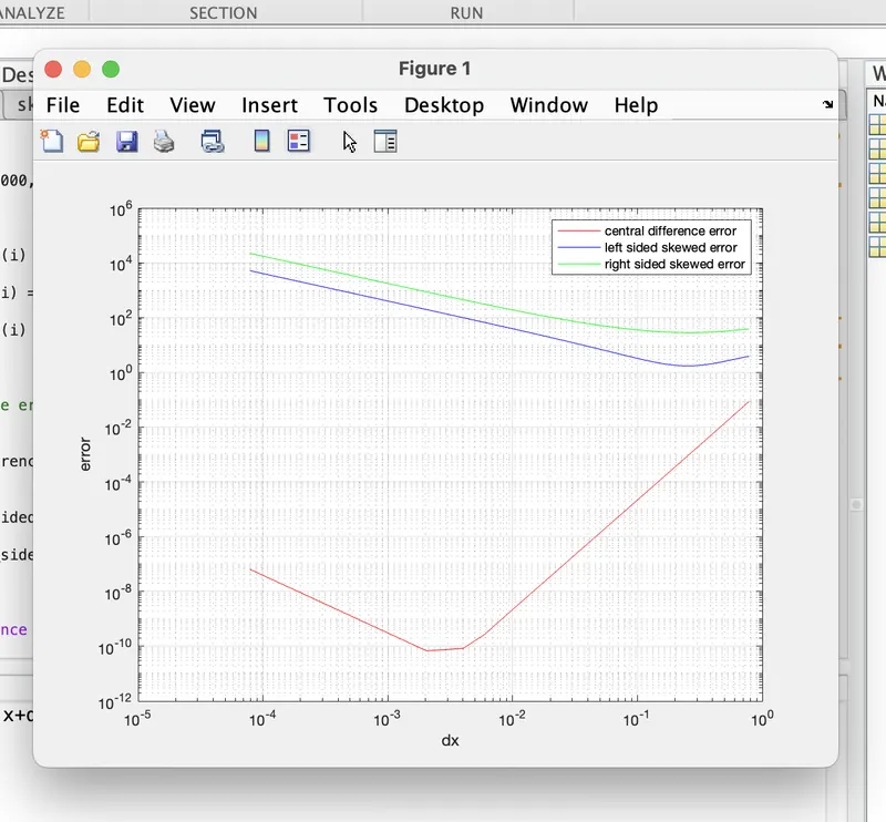
After analysing the graph between 'error' vs. 'dx' for central , skewed left and skewed right sided difference 4th order error , we can easily notice that central difference approximation produces more accurate solutions , hence produces lesser errors as compared to the right -skewed and left -skewed difference schemes.
In your own words, describe why a skewed scheme is useful? What can a skewed scheme do that a CD scheme cannot?
As we can see that the central differencing schemes gives us more accurate solutions with lesser errors as compared to the skewed difference schemes .
But its not always possible to use the central difference to get the solutions.
Suppose if want to compute the numerical approximations for a function at the corner node , at that point or (node) we can't be able to use the central differencing schemes as it requires the input from both the sides of the node , so in this situation skewed difference plays a vital role ; as in the skewed schemes data can be taken from the one side of the node to compute the desired numerical approximation at a point.