Week 5 - Genetic Algorithm

code for finding maxima of the function stalagmite

clc
close all
clear all

x=linspace(0,0.6,150);
y=linspace(0,0.6,150);

[xx yy]=meshgrid(x,y);

for i=1:length(xx);
    for j=1:length(yy);
        input_array(1)=xx(i,j);
        input_array(2)=yy(i,j);
        f(i,j)=stalagmite(input_array);
    end
end

surfc(xx,yy,f)
xlabel('xx')
ylabel('yy')
zlabel('f')

shading interp

[input,funct_val]=ga(@stalagmite,2)
x=input(1)
y=input(2)

code for function stalagmite

function f=stalagmite(input_array)

x=input_array(1);
y=input_array(2);

f_1x=(sin((5.1*pi*x)+0.5))^6;
f_1y=(sin((5.1*pi*y)+0.5))^6;
f_2x=exp(-4*log(2)*(x-0.0667)^2/0.64);
f_2y=exp(-4*log(2)*(y-0.0667)^2/0.64);

f=-(f_1x*f_1y*f_2x*f_2y);

end

explanation for the code above

• first an array of values for x and y using linspace command.
• form sqaure matrix using meshgrid function for x and y denoted as xx and yy.
• each elements of sqare matrix of x and y are given to a row matrix of 2 column.
• each row values for xx and yy are given to a function 'stalagmite'.
• in stalagmite function,we give corresponding formulas and derive value for 'f'.
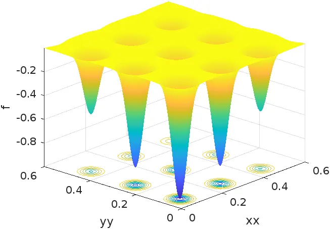
• using surfc command plot a 3d graph of peaks like structure.
• for finding the maximum value by finding optimum value for x and y using genatic algorithm inbuild function.
• thus we get a optimum value for x and y and also maximum value for function 'stalagmite'.

result for the following code

code for finding statistic of values of x and y for 'num' number of times

clc
close all
clear all

x=linspace(0,0.6,150);
y=linspace(0,0.6,150);
num=50;
[xx,yy]=meshgrid(x,y);
for i=1:length(xx);
    for j=1:length(yy);
        input_array(1)=xx(i,j);
        input_array(2)=yy(i,j);
        f(i,j)=stalagmite(input_array);
    end
end

tic
for i=1:num;
    [input,f_opt(i)]=ga(@stalagmite,2);
    x_opt(i)=input(1);
    y_opt(i)=input(2);
end
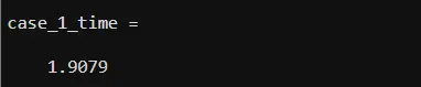
case_1_time=toc

figure(1)
subplot(2,1,1)
hold on
surfc(xx,yy,f)
shading interp
plot3(x_opt,y_opt,f_opt,'marker','o','markersize',5,'markerfacecolor','g')
xlabel('x_opt')
ylabel('y_opt')
zlabel('f_opt')
title('unbounded inputs')
subplot(2,1,2)
plot(f_opt)
xlabel('iteration')
ylabel('function minimum')

%study 2 giving bound to x and y value
tic
for i=1:num;
    [input,f_opt(i)]=ga(@stalagmite,2,[],[],[],[],[0;0],[0.6;0.6]);
    x_opt(i)=input(1);
    y_opt(i)=input(2);
end
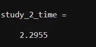
study_2_time=toc

figure(2)
subplot(2,1,1)
hold on
surfc(xx,yy,f)
shading interp
plot3(x_opt,y_opt,f_opt,'marker','o','markersize',5,'markerfacecolor','g')
xlabel('x_opt')
ylabel('y_opt')
zlabel('f_opt')
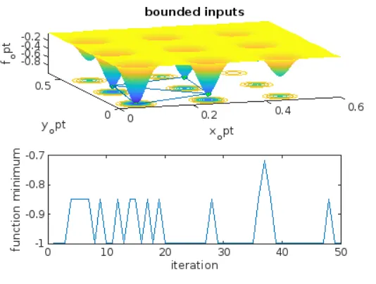
title('bounded inputs')
subplot(2,1,2)
plot(f_opt)
xlabel('iteration')
ylabel('function minimum')

%study 3 increase ga iteration
options=optimoptions('ga');
options=optimoptions(options,'populationsize',400);

tic
for i=1:num
    [input,f_opt(i)]=ga(@stalagmite,2,[],[],[],[],[0;0],[0.6;0.6],[],[],options);
    x_opt(i)=input(1);
    y_opt(i)=input(2);
end
study_3_time=toc

figure(3)
subplot(2,1,1)
hold on
surfc(xx,yy,f)
shading interp
plot3(x_opt,y_opt,f_opt,'marker','o','markersize',5,'markerfacecolor','g')
xlabel('x_opt')
ylabel('y_opt')
zlabel('f_opt')
title('bounded inputs')
subplot(2,1,2)
plot(f_opt)
xlabel('iteration')
ylabel('function minimum')

explanation for the above code

• just like the above function we define values for xand y.subsequently find the value for f.
• usally the value for optimum value of x,y and function value would change for each time.
• so we here going to find the optimum value of x,y and function value for 'num' number of time usingfor loop.
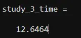
• also we count the time taken to obtaining the optimum solution for 'num' number of times.
• then we going to plot 3 graph in one window using subplot command.
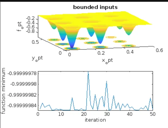
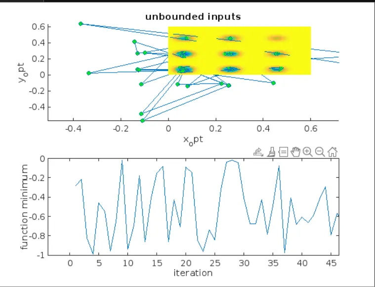
• we plot optimum value of x,y and function value for 'num' number of time using plot3 command and surfc graph in top side of window and at bottom; value of maximum value for function 'stalagmite' is plotted against 'num' number of iteration.
• each point of maximum value for 'stalagmite' in plot3 graph is marked with a sphere of size 5 and color green.
• in second study, we use a bound for values of x and y lies between 0 to 0.6.
• then we plot same types of graph as mentioned above.
• in third study, we increase the number of iteration.
• by this the chances for getting optimum solution would be more.but the time taken to solve this genatic algorithm would take more time compared to rest of two above.

result for the above code

• unbounded normal iteration,surfc graph and optimum solution for x,y and f

• bounded normal iteration,surfc graph and optimum solution for x,y and f

• bounded normal iteration with increase in number of iteration,surfc graph and optimum solution for x,y and f