Week 5 - Genetic Algorithm

AIM:

To Write a code in MATLAB to optimise the stalagmite function and find the global maxima of the function using genetic algorithm.

OBJECTIVE:

• To Write a code in MATLAB to optimise the stalagmite function and find the global maxima of the function using genetic algorithm
• To study the concept of genetic algorithm and also the syntax for ga in MATLAB in your report.
• To Plot graphs for all 3 studies and for F maximum vs no. of iterations.

FORMULA USED:

f1=(sin((5.1*pi*x)+0.5))^6;
f2=(sin((5.1*pi*y)+0.5))^6;
f3=exp((-4)*(log(2))*((x-0.0667)^2/0.64));
f4=exp((-4)*(log(2))*((y-0.0667)^2/0.64));

F=-(f1*f2*f3*f4)

THEORY:

Stalagmite:

The Stalagmite function is a model which is used to generate local minima and maxima.

Genetic Algorithm :

The genetic algorithm is a method for solving both constrained and unconstrained optimization problems that is based on natural selection.The genetic algorithm repeatedly modifies a population of individual solutions. You can apply the genetic algorithm to solve a variety of optimization problems that are not well suited for standard optimization algorithms, including problems in which the objective function is discontinuous, nondifferentiable, stochastic, or highly nonlinear. The genetic algorithm can address problems of mixed integer programming.

Three main types of rules to create the next generation from the current population used in genetic algorithm:

• Selection rules ,

• Crossover rules ,

• Mutation rules .

Working of Ga:

*The algorithm begins by creating a random initial population.

*The algorithm then creates a sequence of new populations. At each step, the algorithm uses the individuals in the current generation to create the next population. To create the new population, the algorithm performs the following steps:

1. Scores each member of the current population by computing its fitness value. These values are called the raw fitness scores.

2. Scales the raw fitness scores to convert them into a more usable range of values. These scaled values are called expectation values.

3. Selects members, called parents, based on their expectation.

4. Some of the individuals in the current population that have lower fitness are chosen as elite. These elite individuals are passed to the next population.

5. Produces children from the parents. Children are produced either by making random changes to a single parent—mutation—or by combining the vector entries of a pair of parents—crossover.

6. Replaces the current population with the children to form the next generation.

*The algorithm stops when one of the stopping criteria is met.

syntax used:

x=ga(@fun,nvars,A,B,Aeq,Beq,Lb,Ub,nonlcon,intcon,options)

• fun= The fitness function in our case the Stalagmite function.
• nvars= number of variables (2)
• A and B= Linear inequalities of the Form A*x<=B
• Aeq and Beq=Linear equalities of the form A*x=B
• LB and UB=Lower and Upper bound that is the region in which Ga will search for the result.
• nonlcon=non Linear inequalities
• intcon=Integer constrained
• options= Helps to add constrain tolerance by increasing the population size.

Main code:

%study 1-satistical behavior:
clear all
close all
clc

x=linspace(0,0.6,150);
y=linspace(0,0.6,150);
num_case=50
[xx,yy]=meshgrid(x,y);
for i=1:length(xx)
for j=1:length(yy)
input_vector(1)=xx(i,j);
input_vector(2)=yy(i,j);
f(i,j)=stalagmite(input_vector);
end
end

tic
for k=1:num_case
[inputs, fopt(k)]=ga(@stalagmite,2);
xopt(k)=inputs(1);
yopt(k)=inputs(2);
end

study1_time=toc

figure(1)
subplot(2,1,1)
surfc(xx,yy,-f)
hold on
shading interp
plot3(xopt,yopt,-fopt,'marker','o','markersize',5,'markerfacecolor','r')
title('Unbounded inputs')
xlabel('X-axis')
ylabel('Y-axis')
subplot(2,1,2)
plot(-fopt)
xlabel('Iterations')
ylabel('Function Maxima')

%study 2- satistical behavior by upper and lower bounds:

tic
for k=1:num_case
[inputs, fopt(k)]=ga(@stalagmite,2,[],[],[],[],[0;0],[1;1]);
xopt(k)=inputs(1);
yopt(k)=inputs(2);
end

study2_time=toc

figure(2)
subplot(2,1,1)
surfc(xx,yy,-f)
hold on
shading interp
plot3(xopt,yopt,-fopt,'marker','o','markersize',5,'markerfacecolor','r')
title('Unbounded inputs')
xlabel('X-axis')
ylabel('Y-axis')
subplot(2,1,2)
plot(-fopt)
xlabel('Iterations')
ylabel('Function Maxima')

%study 3, increasing ga iteration:

tic
for k=1:num_case
[inputs, fopt(k)]=ga(@stalagmite,2,[],[],[],[],[0;0],[1;1],[],[]);
xopt(k)=inputs(1);
yopt(k)=inputs(2);
end

study3_time=toc

figure(3)
subplot(2,1,1)
surfc(xx,yy,-f)
hold on
shading interp
plot3(xopt,yopt,-fopt,'marker','o','markersize',5,'markerfacecolor','r')
title('Unbounded inputs')
xlabel('X-axis')
ylabel('Y-axis')
subplot(2,1,2)
plot(-fopt)
xlabel('Iterations')
ylabel('Function Maxima')

CODE EXPLANATION:

i)

* Creating a function with function definition 'F', and function name as 'stalagmite'.

* the inputs are givens as input vector(1) and input vector(2).

* A formulas are added in the function.

* basically, clear all, close all ,clc is used to clear all the variables and plot which is already exist,

* using linspace command x and y inputs are given and it is convertesd into 2D array using meshgrid command.

* using the nested for loop with i,j as variables and input vector(1), input vector(2) as inputs we are calling the function stalagmite.

ii)study-1

* using the simple statistical behaviour of genetic algorithm we are try to create the local maxima of stalagmite function with given population 50.

* And using plot command we are ploting the inputs of ga function and we are also ploting the F maximum vs no. of iterations using the F function in ga.

* The creation of more local maximum point is not satisfied in the study-1.

iii)study-2

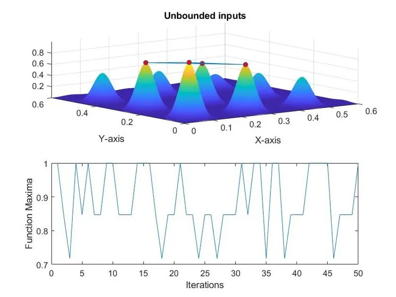
*using the satistical behavior by upper and lower bounds of ga by providing the boundry limits based the graph in the study-1.

* And using plot command we are ploting the inputs of ga function and we are also ploting the F maximum vs no. of iterations using the F function in ga.

* The creation of local maximum point is less(4 to 5 points only) when compaired to the study-1 and the graph also better.

iv)study-3

* By incresing the population (untill we get global max value) of ga function by using optimoptions and populationsize command we are again exiting the ga function.

* And using plot command we are ploting the inputs of ga function and we are also ploting the F maximum vs no. of iterations using the F function in ga.

* we got accurate gobal maximum value by using populationsize of 500.

OUTPUT:

STUDY CASE 1:

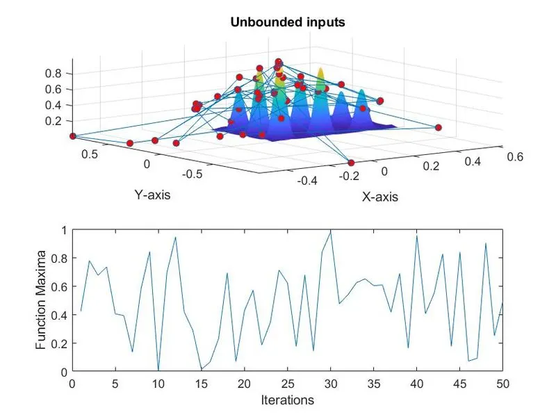
STUDY CASE 2:

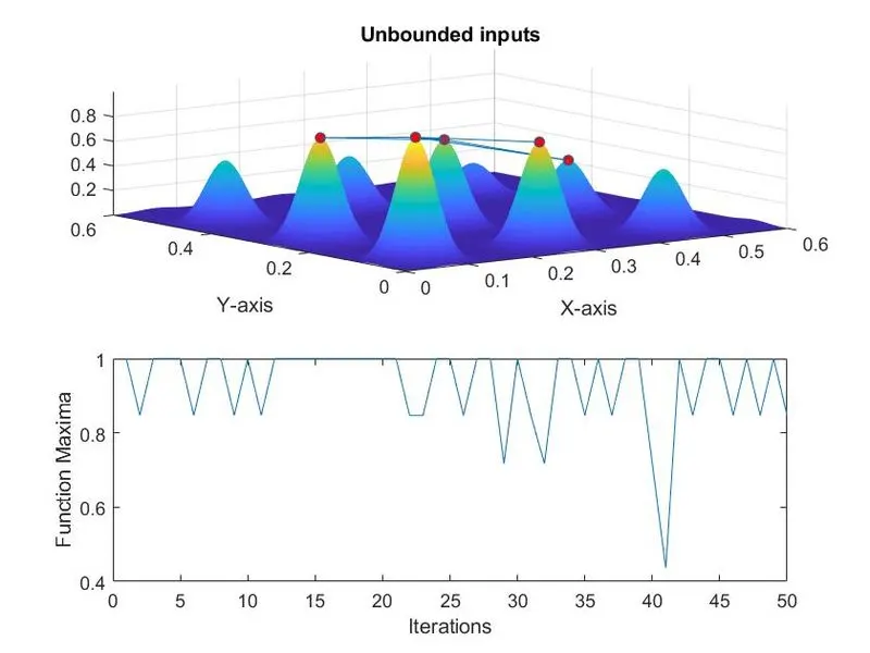
STUDY CASE 3: