Week 5.1 - Mid term project - Solving the steady and unsteady 2D heat conduction problem

CHALLENGE REPORT:

AIM:

To solve the 2D heat conduction equation by using the point iterative techniques by Steady state analysis & Transient State Analysis

OBJECTIVE:

* To solve the 2D heat conduction equation by using the point iterative techniques by Steady state analysis & Transient State Analysis.

* Implement the methods for solving implicit equations.

1. Jacobi

2. Gauss-seidel

3. Successive over-relaxation

* Write code for both implicit and explicit schemes

THEORY :

The heat conduction equation can be solved in two ways

1. Steady state

2. Transient state

STEADY STATE :

Solving 2D steady state heat conduction equation

Here the time term gets eliminated ie, (∂T)/(∂t)=0

`(∂T)/(∂t)=0`

so the eqution becomes,(∂^2 T)/(∂x^2 )+(∂^2 T)/(∂y^2 )=0

This equation is of elliptic in nature so the informations are taken from the surroundings,

hence we can write the eqution as follows:

(T_L-2T_P+T_R)/(Δx^2 )+(T_T-2T_p+T_B)/(Δy^2 )=0

if we put K =2(Δx^2+Δy^2 )/(Δx^2⋅Δy^2 )

we can write the expression for T_p from the above equation as:

T_p=1/k ((T_L+T_R)/(Δx^2 )+(T_T+T_B)/(Δy^2 ))

The above equation is used for itration .

1. Jacobi method

In numerical linear algebra, the Jacobi method is an iterative algorithm for determining the solutions of a strictly diagonally dominant system of linear equations. Each diagonal element is solved for, and an approximate value is plugged in. The process is then iterated until it converges.

2. Gauss siedel method

Gauss–Seidel method is an iterative method to solve a set of linear equations and very much similar to Jacobi’s method. This method is also known as Liebmann method or the method of successive displacement. The name successive displacement is because the second unknown is determined from the first unknown in the current iteration, the third unknown is determined from the first and second unknowns.

3. Successive over relaxed method

The method of successive over relaxation (SOR) is a variant of the Gauss-siedel method for solving a linear system of equations, resulting in faster convergence. A similar method can be used for any slowly converging iterative process.

CODE FOR STEADY STATE :

clear all
close all
clc

%inputs
L=1;
nx=20;
ny=20;
tolerance=1e-4;
error=1000;
iterative_solver=input('enter the solver number:')

%function for steady state jacobi method
if iterative_solver==1
steady_state_2D_jacobi_method(L,nx,ny,tolerance,error);
end

if iterative_solver==2
steady_state_2D_gauss_seidal_method(L,nx,ny,tolerance,error);
end

if iterative_solver==3
steady_state_2D_SOR_method(L,nx,ny,tolerance,error);
end

Function steady state by Jacobi method:
function [T,jacobi]=steady_state_2D_jacobi_method(L,nx,ny,tolerance,error)
tic
x=linspace(0,L,nx);
y=linspace(0,L,ny);
dx=L/(nx-1);
dy=L/(ny-1);
%temperatutre matrix
T=300*ones(nx,ny);
T_r=800;
T_l=400;
T_t=600;
T_b=900;

T(:,1)=T_l;
T(:,end)=T_r;
T(1,:)=T_t;
T(end,:)=T_b;

%edges
T(1,1)=(T_l+T_t)/2;
T(1,end)=(T_t+T_r)/2;
T(end,1)=(T_l+T_b)/2;
T(end,end)=(T_b+T_r)/2;
k=(2*((dx)^2+(dy)^2))/((dx)^2*(dy)^2);
Told=T;
j_iteration_no=1;
%loop
while (error>tolerance)
for i=2:(nx-1)
for j=2:(ny-1)
T(i,j)=(1/k)*(((Told(i-1,j)+Told(i+1,j))/(dx^2))+((Told(i,j-1)+Told(i,j+1))/(dy^2)));
end
end
error=max(max(abs(Told-T)));
Told=T;
j_iteration_no=j_iteration_no+1;

%plot

end
figure(1)
contourf(x,y,T,'showtext','on')
set(gca,'ydir','reverse')
colormap(jet);
colorbar;
time_count_jaco=toc;
tittle_text=sprintf('steady state 2D heat conduction jacobi iteration_no=%d time=%f s',j_iteration_no, time_count_jaco);
title(tittle_text);
xlabel('x axis');
ylabel('y axis');

end

function steady state by Gauss siedel method:

function [T,gauss]=steady_state_2D_gauss_seidal_method(L,nx,ny,tolerance,error)
tic
x=linspace(0,L,nx);
y=linspace(0,L,ny);
dx=L/(nx-1);
dy=L/(ny-1);
%temperatutre matrix
T=300*ones(nx,ny);
T_r=800;
T_l=400;
T_t=600;
T_b=900;

T(:,1)=T_l;
T(:,end)=T_r;
T(1,:)=T_t;
T(end,:)=T_b;

%edges
T(1,1)=(T_l+T_t)/2;
T(1,end)=(T_t+T_r)/2;
T(end,1)=(T_l+T_b)/2;
T(end,end)=(T_b+T_r)/2;
k=(2*((dx)^2+(dy)^2))/((dx)^2*(dy)^2);
Told=T;
Ga_iteration_no=1;
%loop
while (error>tolerance)
for i=2:(nx-1)
for j=2:(ny-1)
T(i,j)=(1/k)*(((T(i-1,j)+Told(i+1,j))/(dx^2))+((T(i,j-1)+Told(i,j+1))/(dy^2)));
end
end
error=max(max(abs(Told-T)));
Told=T;
Ga_iteration_no=Ga_iteration_no+1;

%plot

end
figure(2)
contourf(x,y,T)
set(gca,'ydir','reverse')
colormap(jet);
colorbar;
time_count_gauss=toc;
tittle_text=sprintf('steady state 2D heat conduction gauss iteration_no=%d time=%f s',Ga_iteration_no,time_count_gauss);
title(tittle_text);
xlabel('x axis');
ylabel('y axis');

end

function steady state by SOR method:

function [T,SOR]=steady_state_2D_SOR_method(L,nx,ny,tolerance,error)
tic
x=linspace(0,L,nx);
y=linspace(0,L,ny);
dx=L/(nx-1);
dy=L/(ny-1);
%temperatutre matrix
T=300*ones(nx,ny);
T_r=800;
T_l=400;
T_t=600;
T_b=900;

T(:,1)=T_l;
T(:,end)=T_r;
T(1,:)=T_t;
T(end,:)=T_b;

%edges
T(1,1)=(T_l+T_t)/2;
T(1,end)=(T_t+T_r)/2;
T(end,1)=(T_l+T_b)/2;
T(end,end)=(T_b+T_r)/2;
k=(2*((dx)^2+(dy)^2))/((dx)^2*(dy)^2);
Told=T;
SOR_iteration_no=1;
omaga=1.5;
%loop
while (error>tolerance)
for i=2:(nx-1)
for j=2:(ny-1)
term1=((T(i-1,j)+Told(i+1,j))/(dx^2));
term2=((T(i,j-1)+Told(i,j+1))/(dy^2));
Tg=(1/k)*(term1+term2);
T(i,j)=(1-omaga)*Told(i,j)+omaga*Tg;
% Tga(i,j)=(1/k)*(((T(i-1,j)+Told(i+1,j))/(dx^2))+((T(i,j-1)+Told(i,j+1))/(dy^2)));
% T(i,j)=(1-omaga)*Told(i,j)+omaga*Tga(i,j)
end
end
error=max(max(abs(Told-T)));
Told=T;
SOR_iteration_no=SOR_iteration_no+1;

%plot

end
figure(1)
contourf(x,y,T)
set(gca,'ydir','reverse')
colormap(jet);
colorbar;
time_count_SOR=toc;
tittle_text=sprintf('steady state 2D heat conduction SOR iteration_no=%d time=%f s',SOR_iteration_no, time_count_SOR);
title(tittle_text);
xlabel('x axis');
ylabel('y axis');

end

CODE EXPLANATION:

* clear all, close all, clc is used to clear all the variables and the figure which is created already.

* Assign the inputs length as L, nx=20, ny=20 and tolerance=1e-4, error=1000.

* And create if condition with iterative solver==1 or 2 or 3 as condition and assign the function for jacobian, gauss siedel, SOR method which as be created.

* Function for Jacobian method,

A function is created with [T,jacobi] as function definition and steady_state_2D_jacobi_method(L,nx,ny,tolerance,error) as the function name.

* In that assign the inputs for x, y, dx, dy, T and add the boundary condition given (T_r=800; T_l=400; T_t=600; T_b=900)

* Assign the edges using the given boundary conditions ( T(1,1)=(T_l+T_t)/2; T(1,end)=(T_t+T_r)/2; T(end,1)=(T_l+T_b)/2; T(end,end)=(T_b+T_r)/2 )

* Make Told equal to T and give initial jacobian iterative no as 1 and assign the k variable from the steady state formula.

* Create a while loop as error>tolerance as condition and in that create for loop with 'i' as variable range from 2 to nx-1 and create another for loop with 'j' as variable range from 2 to ny-1 and assign the jacobi formula based on the steady state equations [ T(i,j)=(1/k)*(((Told(i-1,j)+Told(i+1,j))/(dx^2))+((Told(i,j-1)+Told(i,j+1))/(dy^2))) ]and end the two for loops.

* Give error=max(max(abs(Told-T))) and Told equal to T and j_iteration_no=j_iteration_no+1 before ending the while loop an dend it.

* Using the contourf command is used to plot the graph and colormap(jet) is used to give bright colour nad color bar is used to colour it aned added wit tittle , xlabel, ylabel and end the function.

* Function for Gauss siedel method,

A function is created with [T,Gauss] as function definition and steady_state_2D_Gauss_siedel_method(L,nx,ny,tolerance,error) as the function name.

* In that assign the inputs for x, y, dx, dy, T and add the boundary condition given (T_r=800; T_l=400; T_t=600; T_b=900)

* Assign the edges using the given boundary conditions ( T(1,1)=(T_l+T_t)/2; T(1,end)=(T_t+T_r)/2; T(end,1)=(T_l+T_b)/2; T(end,end)=(T_b+T_r)/2 )

* Make Told equal to T and give initial Gauss iterative no as 1 and assign the k variable from the steady state formula.

* Create a while loop as error>tolerance as condition and in that create for loop with 'i' as variable range from 2 to nx-1 and create another for loop with 'j' as variable range from 2 to ny-1 and assign the formula based on the steady state equations [ T(i,j)=(1/k)*(((T(i-1,j)+Told(i+1,j))/(dx^2))+((T(i,j-1)+Told(i,j+1))/(dy^2))) ]and end the two for loops.

* Give error=max(max(abs(Told-T))) and Told equal to T and Gauss_iteration_no=Gauss_iteration_no+1 before ending the while loop an dend it.

* Using the contourf command is used to plot the graph and colormap(jet) is used to give bright colour nad color bar is used to colour it aned added wit tittle , xlabel, ylabel and end the function.

* Function for SOR method,

A function is created with [T,SOR] as function definition and steady_state_2D_SOR_method(L,nx,ny,tolerance,error) as the function name.

* In that assign the inputs for x, y, dx, dy, T and add the boundary condition given (T_r=800; T_l=400; T_t=600; T_b=900)

* Assign the edges using the given boundary conditions ( T(1,1)=(T_l+T_t)/2; T(1,end)=(T_t+T_r)/2; T(end,1)=(T_l+T_b)/2; T(end,end)=(T_b+T_r)/2 ) and omaga=1.5.

* Make Told equal to T and give initial SOR iterative no as 1 and assign the k variable from the steady state formula.

* Create a while loop as error>tolerance as condition and in that create for loop with 'i' as variable range from 2 to nx-1 and create another for loop with 'j' as variable range from 2 to ny-1 and assign the formula based on the steady state equations [ T(i,j)=(1-omaga)*Told(i,j)+omaga*Tg ]and end the two for loops.

* Give error=max(max(abs(Told-T))) and Told equal to T and SOR_iteration_no=SOR_iteration_no+1 before ending the while loop an dend it.

* Using the contourf command is used to plot the graph and colormap(jet) is used to give bright colour nad color bar is used to colour it aned added wit tittle , xlabel, ylabel and end the function.

PLOTS:

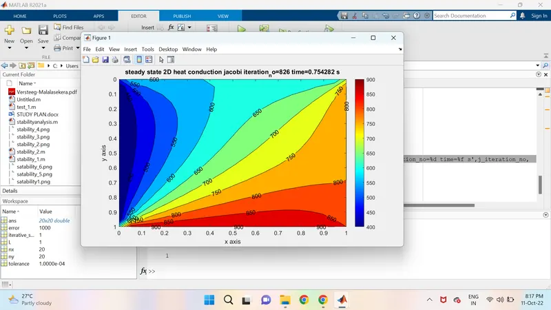
1. Jacobian method:

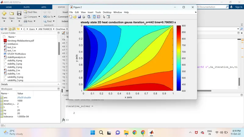
2.Gauss siedel:

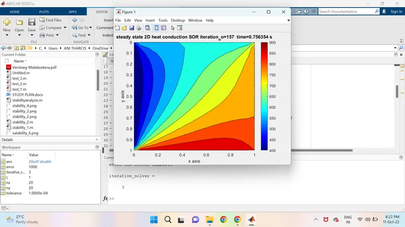
3.SOR method:

Results :

As you can see from the above results Jacobi method has the highest number of iteration with an elapsed time of 490.96 seconds. Gauss-siedel method has less number of iterations than jacobi method .Also it can be seen that SOR method is most efficient since it hace less number of iteration and the elapsed time is very less. The SOR method really depend on the relaxation factor which I used here as omega (w) .

TRANSIENT :

In transient state there are two scheme ,

* Implicit and

* Explicit.

Transient Implicit scheme :

Working principle of the Implicit Scheme:

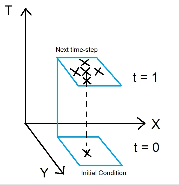
* We have a matrix with the boundary conditions and the initial conditions at time t = 0 as shown in the above image.

* Now, if we need to calculate the value of a node in the next matrix at time t = 1, the implicit formulation requests the value of that particular node from its previous position at the first matrix which is at the time t = 0.

* Now, if we want to calculate the values of the neighboring nodes of the previous node at t = 1, we have to consider them as unknowns as here only the value of the node at a time, t = 0 is known to us.

* So, we have 5 unknowns right now.

* When we try to write the equations for all the terms, we get a series of unknowns like this in such a way that we have a system of equations for every node.

* So it results in the formulation of a system like this one: A*X = B

* Here A is the 'Coefficient', B is the 'Boundary Conditions' and X is the 'Unknowns'.

* This is what we are trying to solve iteratively same as in our steady-state code by using various iterative solvers like Jacobi, GS, and SOR.

* Here, iterations take place at each of the time steps. To find out the values of nodes at each matrix for varying time steps we have to write code so that the current matrix considers the value of its nodes from the previous matrix at the previous time step and takes the matrix further upwards in time.

* We can consider the number of time steps to be 'nt'. So we have to use a criterion to denote the number of time steps it will go up for.

* We have to then calculate the number of iterations it takes for the equations to converge at each time step.

CODE FOR TRANSIENT IMPLICIT :

clear all
close all
clc

%inputs
L=1;
nx=20;
ny=20;
tolerance=1e-4;
% error=1000;
iterative_solver=input('enter the solver number:')

%function for steady state jacobi method
if iterative_solver==1
transint_implicit_2D_jacobi_method(L,nx,ny,tolerance)
end

if iterative_solver==2
transint_implicit_2D_gauss_seidal_method(L,nx,ny,tolerance)
end

if iterative_solver==3
transint_implicit_2D_SOR_method(L,nx,ny,tolerance)
end

function for Jacobian by SOR method:
function [T,jacobi]=transint_implicit_2D_jacobi_method(L,nx,ny,tolerance)
tic
x=linspace(0,L,nx);
y=linspace(0,L,ny);
dx=L/(nx-1);
dy=L/(ny-1);
dt=1e-4;
nt=1400;
alpha=1.4;
%temperatutre matrix
T=300*ones(nx,ny);
T_r=800;
T_l=400;
T_t=600;
T_b=900;

T(:,1)=T_l;
T(:,end)=T_r;
T(1,:)=T_t;
T(end,:)=T_b;

%edges
T(1,1)=(T_l+T_t)/2;
T(1,end)=(T_t+T_r)/2;
T(end,1)=(T_l+T_b)/2;
T(end,end)=(T_b+T_r)/2;
k1=(alpha*dt)/(dx^2);
k2=(alpha*dt)/(dy^2);
k3=1/(1+2*k1+2*k2);
Told=T;
Tpre=T;
j_iteration_no=1;
%loop
for z=1:nt
error =1000;
while (error>tolerance)
for i=2:(nx-1)
for j=2:(ny-1)
T(i,j)=k3*(Tpre(i,j)+(k1*(Told(i-1,j)+Told(i+1,j))+(k2*(Told(i,j-1)+Told(i,j+1)))));
end
end
error=max(max(abs(Told-T)));
Told=T;
j_iteration_no=j_iteration_no+1;
Tpre=T;

%plot

end
end
figure(1)
contourf(x,y,T,'showtext','on')
set(gca,'ydir','reverse')
colormap(jet);
colorbar;
time_count_jaco=toc;
tittle_text=sprintf('steady state 2D heat conduction jacobi iteration_no=%d time=%f s',j_iteration_no, time_count_jaco);
title(tittle_text);
xlabel('x axis');
ylabel('y axis');

end

function for Transient by Gauss siedel method:

function [T,gauss]=transint_implicit_2D_gauss_seidal_method(L,nx,ny,tolerance)
tic
x=linspace(0,L,nx);
y=linspace(0,L,ny);
dx=L/(nx-1);
dy=L/(ny-1);
dt=1e-4;
nt=1400;
alpha=1.4;
%temperatutre matrix
T=300*ones(nx,ny);
T_r=800;
T_l=400;
T_t=600;
T_b=900;

T(:,1)=T_l;
T(:,end)=T_r;
T(1,:)=T_t;
T(end,:)=T_b;

%edges
T(1,1)=(T_l+T_t)/2;
T(1,end)=(T_t+T_r)/2;
T(end,1)=(T_l+T_b)/2;
T(end,end)=(T_b+T_r)/2;
k1=(alpha*dt)/(dx^2);
k2=(alpha*dt)/(dy^2);
k3=1/(1+2*k1+2*k2);
Told=T;
Tpre=T;
gauss_iteration_no=1;
%loop
for z=1:nt
error =1000;
while (error>tolerance)
for i=2:(nx-1)
for j=2:(ny-1)
T(i,j)=k3*(Tpre(i,j)+(k1*(T(i-1,j)+Told(i+1,j))+(k2*(T(i,j-1)+Told(i,j+1)))));
end
end
error=max(max(abs(Told-T)));
Told=T;
gauss_iteration_no=gauss_iteration_no+1;
Tpre=T;

%plot

end
end
figure(1)
contourf(x,y,T,'showtext','on')
set(gca,'ydir','reverse')
colormap(jet);
colorbar;
time_count_gauss=toc;
tittle_text=sprintf('steady state 2D heat conduction gauss iteration_no=%d time=%f s',gauss_iteration_no, time_count_gauss);
title(tittle_text);
xlabel('x axis');
ylabel('y axis');

end

function for Transient by SOR method:

function [T,jacobi]=transint_implicit_2D_SOR_method(L,nx,ny,tolerance)
tic
x=linspace(0,L,nx);
y=linspace(0,L,ny);
dx=L/(nx-1);
dy=L/(ny-1);
dt=1e-4;
nt=1400;
alpha=1.4;
%temperatutre matrix
T=300*ones(nx,ny);
T_r=800;
T_l=400;
T_t=600;
T_b=900;

T(:,1)=T_l;
T(:,end)=T_r;
T(1,:)=T_t;
T(end,:)=T_b;

%edges
T(1,1)=(T_l+T_t)/2;
T(1,end)=(T_t+T_r)/2;
T(end,1)=(T_l+T_b)/2;
T(end,end)=(T_b+T_r)/2;
k1=(alpha*dt)/(dx^2);
k2=(alpha*dt)/(dy^2);
k3=1/(1+2*k1+2*k2);
omaga=1.5;
Told=T;
Tpre=T;
SOR_iteration_no=1;
%loop
for z=1:nt
error =1000;
while (error>tolerance)
for i=2:(nx-1)
for j=2:(ny-1)
Tga=k3*(Tpre(i,j)+(k1*(T(i-1,j)+Told(i+1,j))+(k2*(T(i,j-1)+Told(i,j+1)))));
T(i,j)=(1-omaga)*Told(i,j)+omaga*(Tga);
end
end
error=max(max(abs(Told-T)));
Told=T;
SOR_iteration_no=SOR_iteration_no+1;
Tpre=T;

%plot

end
end
figure(1)
contourf(x,y,T,'showtext','on')
set(gca,'ydir','reverse')
colormap(jet);
colorbar;
time_count_jaco=toc;
tittle_text=sprintf('steady state 2D heat conduction SOR iteration_no=%d time=%f s',SOR_iteration_no, time_count_jaco);
title(tittle_text);
xlabel('x axis');
ylabel('y axis');

end

CODE EXPLANATION:

* clear all, close all, clc is used to clear all the variables and the figure which is created already.

* Assign the inputs length as L, nx=20, ny=20 and tolerance=1e-4.

* And create if condition with iterative solver==1 or 2 or 3 as condition and assign the function for jacobian, gauss siedel, SOR method which as be created.

* Function for Jacobian method,

A function is created with [T,jacobi] as function definition and TRanient_implicit_2D_jacobi_method(L,nx,ny,tolerance) as the function name.

* In that assign the inputs for x, y, dx, dy, T and add the boundary condition given (T_r=800; T_l=400; T_t=600; T_b=900)

* Assign the edges using the given boundary conditions ( T(1,1)=(T_l+T_t)/2; T(1,end)=(T_t+T_r)/2; T(end,1)=(T_l+T_b)/2; T(end,end)=(T_b+T_r)/2 )

* Make Told equal to T and give initial jacobian iterative no as 1 and assign the k variable from the steady state formula.

* Create a for loop with z as variable range from 1 to nt and assign , error=1000 and create while loop as error>tolerance as condition and in that create for loop with 'i' as variable range from 2 to nx-1 and create another for loop with 'j' as variable range from 2 to ny-1 and assign the jacobi formula based on the Transient implicit equations [ T(i,j)=k3*(Tpre(i,j)+(k1*(Told(i-1,j)+Told(i+1,j))+(k2*(Told(i,j-1)+Told(i,j+1)))) ]and end the two for loops.

* Give error=max(max(abs(Told-T))) and Told equal to T and j_iteration_no=j_iteration_no+1 before ending the while loop an dend it.

* Using the contourf command is used to plot the graph and colormap(jet) is used to give bright colour nad color bar is used to colour it aned added wit tittle , xlabel, ylabel and end the function.

* Function for Gauss siedel method,

A function is created with [T,Gauss] as function definition and Transient_implicit_2D_Gauss_siedel_method(L,nx,ny,tolerance,error) as the function name.

* In that assign the inputs for x, y, dx, dy, T and add the boundary condition given (T_r=800; T_l=400; T_t=600; T_b=900)

* Assign the edges using the given boundary conditions ( T(1,1)=(T_l+T_t)/2; T(1,end)=(T_t+T_r)/2; T(end,1)=(T_l+T_b)/2; T(end,end)=(T_b+T_r)/2 )

* Make Told equal to T and give initial Gauss iterative no as 1 and assign the k variable from the steady state formula.

* Create a for loop with z as variable range from 1 to nt and assign , error=1000 and create while loop as error>tolerance as condition and in that create for loop with 'i' as variable range from 2 to nx-1 and create another for loop with 'j' as variable range from 2 to ny-1 and assign the formula based on the Transient implicit equations [ T(i,j)=k3*(Tpre(i,j)+(k1*(T(i-1,j)+Told(i+1,j))+(k2*(T(i,j-1)+Told(i,j+1)))) ]and end the two for loops.

* Give error=max(max(abs(Told-T))) and Told equal to T and Gauss_iteration_no=Gauss_iteration_no+1 before ending the while loop an dend it.

* Using the contourf command is used to plot the graph and colormap(jet) is used to give bright colour nad color bar is used to colour it aned added wit tittle , xlabel, ylabel and end the function.

* Function for SOR method,

A function is created with [T,SOR] as function definition and Transient_implicit_2D_SOR_method(L,nx,ny,tolerance,error) as the function name.

* In that assign the inputs for x, y, dx, dy, T and add the boundary condition given (T_r=800; T_l=400; T_t=600; T_b=900)

* Assign the edges using the given boundary conditions ( T(1,1)=(T_l+T_t)/2; T(1,end)=(T_t+T_r)/2; T(end,1)=(T_l+T_b)/2; T(end,end)=(T_b+T_r)/2 ) and omaga=1.5.

* Make Told equal to T and give initial SOR iterative no as 1 and assign the k variable from the steady state formula.

* Create a for loop with z as variable range from 1 to nt and assign , error=1000 and create while loop as error>tolerance as condition and in that create for loop with 'i' as variable range from 2 to nx-1 and create another for loop with 'j' as variable range from 2 to ny-1 and assign the formula based on the Transient Implicit equations [ T(i,j)=(1-omaga)*Told(i,j)+omaga*Tg ]and end the two for loops.

* Give error=max(max(abs(Told-T))) and Told equal to T and SOR_iteration_no=SOR_iteration_no+1 before ending the while loop an dend it.

* Using the contourf command is used to plot the graph and colormap(jet) is used to give bright colour nad color bar is used to colour it aned added wit tittle , xlabel, ylabel and end the function.

PLOTS :

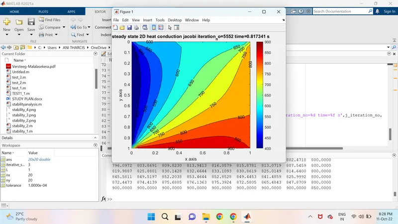
1.Jacobian :

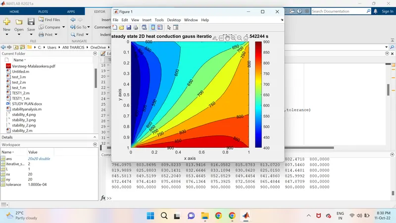
2. Gauss siedel :

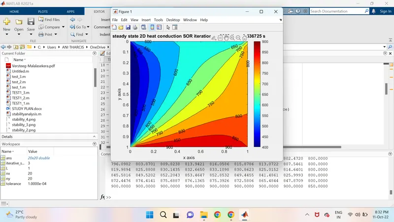
3. SOR METHOD :

Result :

Here we can see that SOR method takes less time and less number of iterations , so SOR method can be defined as efficient method to solve transient heat equation implicitly. Jacobi method again comes up with larger number of iterations and takes more time to calculate.

Transient Explicit Scheme :

Working principle of the Implicit Scheme:

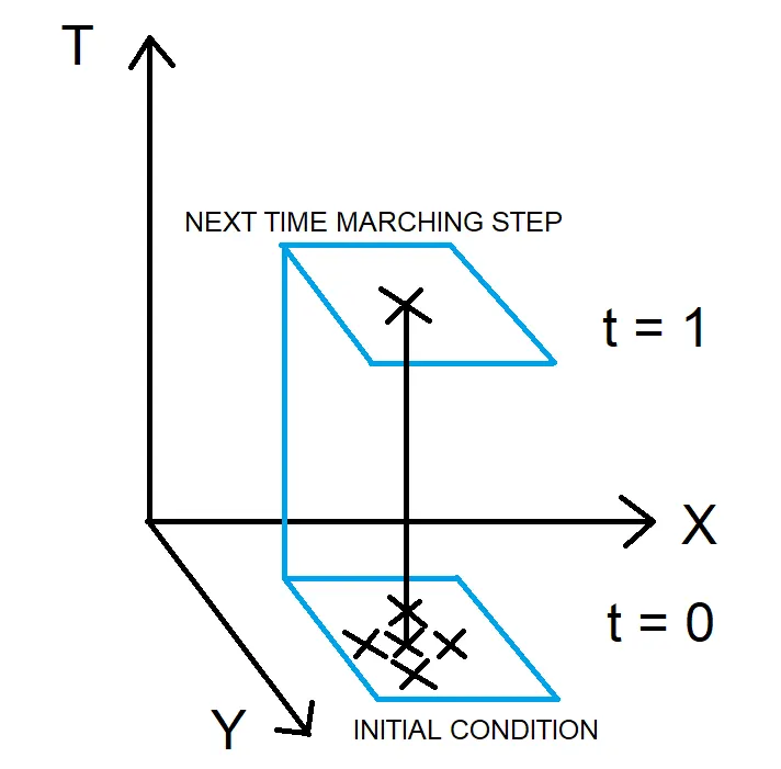
*The Explicit-Scheme tells us that in order to find out the value of the node at the next time step we need the value of that node from its previous matrix and the value of its neighboring nodes.

* The entire matrix is already known to us here and we just have to increment the value of our time.

* We don't require any iterative solvers here as we can reach convergence just by going up in time.

* The only thing we should be concerned about here is how long we need to increase our value of time.

* We can estimate that by using a convergence variable which will enable us to subtract the temperature matrix at the time, t = 0 and t = 1, and so on so that we can compare the value we got after subtracting it with one another and compare it with the value of convergence to determine whether or not it has reached convergence.

* The only iteration present here is for time-iteration.

* Discretization:

* We're then going to state our discretized equation inside the time loop and we're using only Tunderset(prev).

* We don't have a value of error here but rather have a convergence value to compare the plots with.

* We're also introducing a new variable named 'time_iter' which will count the number of times our time iteration's value has been incremented.

* We have to implement an additional parameter called CFL which stands for Courant-Friedrichs-Lewy. CFL is given as k1+k2 here.

* Implicit conditions don't require the CFL parameter. The value of CFL should be less than 0.5 for a 2D system of equations.

* Here, the value of our CFL is 0.1600 which satisfies the above-mentioned condition.

* If the value of CFL increases more than 0.5, it enters divergence instead of convergence.

CODE FOR TRANSIENT EXPLICIT :

clear all
close all
clc
tic
L=1;
nx=20;
ny=20;
tolerance=1e-4;
x=linspace(0,L,nx);
y=linspace(0,L,ny);
dx=L/(nx-1);
dy=L/(ny-1);
dt=4e-4;
nt=1400;
alpha=1.4;
%temperatutre matrix
T=300*ones(nx,ny);
T_r=800;
T_l=400;
T_t=600;
T_b=900;

T(:,1)=T_l;
T(:,end)=T_r;
T(1,:)=T_t;
T(end,:)=T_b;

%edges
T(1,1)=(T_l+T_t)/2;
T(1,end)=(T_t+T_r)/2;
T(end,1)=(T_l+T_b)/2;
T(end,end)=(T_b+T_r)/2;
k1=(alpha*dt)/(dx^2);
k2=(alpha*dt)/(dy^2);

CFL=k1+k2;
Told=T;
Tpre=T;
explicit_iteration_no=1;
%loop
for z=1:nt
conv =1000;
% while (conv>tolerance)
for i=2:(nx-1)
for j=2:(ny-1)
T(i,j)=Told(i,j) + k1*(Told(i-1,j)-2*Told(i,j)+Told(i+1,j)) + k2*(Told(i,j-1)-2*Told(i,j)+Told(i,j+1));
end
end
% conv=max(max(abs(Told-T)));
Told=T;
explicit_iteration_no=explicit_iteration_no+1;
Tpre=T;

%plot

end

figure(1)
contourf(x,y,T,'showtext','on')
set(gca,'ydir','reverse')
colormap(jet);
colorbar;
time_count=toc;
tittle_text=sprintf('steady state 2D heat conduction explicit iteration_no=%d time=%f s',explicit_iteration_no,time_count);
title(tittle_text);
xlabel('x axis');
ylabel('y axis');

CODE EXPLANATION :

* clear all, close all, clc is used to clear all the variables and the figure which is created already.

* Assign the inputs length as L, nx=20, ny=20 and tolerance=1e-4, x, y, dx, dy, T and add the boundary condition given (T_r=800; T_l=400; T_t=600; T_b=900)

* Assign the edges using the given boundary conditions ( T(1,1)=(T_l+T_t)/2; T(1,end)=(T_t+T_r)/2; T(end,1)=(T_l+T_b)/2; T(end,end)=(T_b+T_r)/2 )

* Assign the k variable from the Transient explicit formula and Give CFL=k1+k2 and make Told equal to T and give explicit iterative no as 1.

* Create a for loop with z as variable range from 1 to nt and assign ,conv=1000 and create for loop with 'i' as variable range from 2 to nx-1 and create another for loop with 'j' as variable range from 2 to ny-1 and assign the formula based on the Transient implicit equations [ T(i,j)=Told(i,j) + k1*(Told(i-1,j)-2*Told(i,j)+Told(i+1,j)) + k2*(Told(i,j-1)-2*Told(i,j)+Told(i,j+1)) ]and end the two for loops.

* Give Told equal to T and explicit_iteration_no=j_iteration_no+1 before ending the while loop an dend it.

* Using the contourf command is used to plot the graph and colormap(jet) is used to give bright colour nad color bar is used to colour it aned added wit tittle , xlabel, ylabel and end the function.

PLOT :

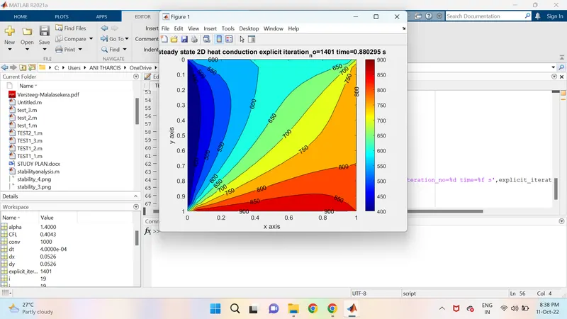
Result :

Explicit is depends on the CFL value

The above plot has a CFL value of less than one as required and hence the Time-Iterations are converging eventually.

If the value of CFL was more than 0.5, then this plot would enter divergence.