Week 5 - Curve fitting

1. What does popt and pcov mean? (Watch the video to get some context)

Answer:

popt is an array that contains the optimal values of the parameters for the fitting model. These values are determined by minimizing the difference between the model's predictions and the actual data. It represents the "best-fit" solution for the given data and the specified model. These parameters minimize the difference between the model's predictions and the actual data.

pcov is the covariance matrix of the parameter estimates contained in popt. It provides a measure of the uncertainty or confidence in the fitted parameters.he diagonal elements of pcov are the variances of the corresponding parameters. Taking the square root of these values gives the standard errors. The diagonal elements of pcov are the variances of the corresponding parameters. Taking the square root of these values gives the standard errors. The off-diagonal elements represent the covariances between pairs of parameters, indicating how changes in one parameter may affect the others.

2. What does np.array(temperature) do?

The function np.array(temperature) converts the Python list temperature into a NumPy array. Efficient Computations enables vectorized operations (e.g., element-wise addition or multiplication). Ensures compatibility with NumPy functions like curve fitting, plotting, or mathematical operations.

3. What does the * in *popt mean?What does the * in *popt mean?

The "*"operator unpacks the elements of an iterable (like a list or array) and passes them as individual arguments to a function. This is commonly used in curve fitting to pass multiple parameters dynamically.

4. Write code to fit a linear and cubic polynomial for the Cp data. Explain if your results are good or bad.

import numpy as np

import matplotlib.pyplot as plt

from scipy.optimize import curve_fit

# curve fit function

def linear(t, a, b):

return a*t + b

# Reading Thermodynamic data file

def read_file():

temperature = []

cp = []

for line in open('data','r'):

values = line.split(',')

temperature.append(float(values[0]))

cp.append(float(values[1]))

return [temperature, cp ]

# Main program

temperature, cp = read_file()

popt_1, pcov_1 = curve_fit(linear, temperature, cp)

fit_cp1 = linear(np.array(temperature), *popt_1)

plt.plot(temperature, cp,color = "blue", linewidth = 3)

plt.plot(temperature, fit_cp1,color ="red", linewidth = 3 )

plt.legend(['Actual data','Curve fit'])

plt.xlabel('temperature [K]')

plt.ylabel('cp')

plt.title("Curve fit for linear polynomial")

plt.show()

#Goodness of Fit characteristic GOF

total_cp = np.sum(cp)

numval_cp = np.size(cp)

avg_cp = total_cp/numval_cp

print('Average Cp is:', avg_cp)

for i in range(numval_cp):

sst = np.sum(pow((cp[i]-avg_cp),2))

ssr = np.sum(pow((cp[i]-fit_cp1[i]),2))

# R-Squared Value

r_squared = 1-(ssr/sst)

print("R-Squared:", r_squared)

# Root Mean Square Error (RMSE)

rmse = pow((ssr/numval_cp),0.5)

print("RMSE:", rmse)

# curve fit function cubic

def cubic(t ,a ,b, c, d):

return a*pow(t,3) + b*pow(t,2) + c*t + d

# Reading Thermodynamic data file

def read_file():

temperature = []

cp = []

for line in open('data','r'):

values = line.split(',')

temperature.append(float(values[0]))

cp.append(float(values[1]))

return [temperature, cp ]

# Main program

temperature, cp = read_file()

popt_1, pcov_1 = curve_fit(cubic, temperature, cp)

fit_cp2 = cubic(np.array(temperature), *popt_1)

plt.plot(temperature, cp,color = "blue", linewidth = 3)

plt.plot(temperature, fit_cp2,color ="red", linewidth = 3 )

plt.legend(['Actual data','Curve fit'])

plt.xlabel('temperature [K]')

plt.ylabel('cp')

plt.title("Curve fit for cubic polynomial")

plt.show()

# Goodness of Fit Characteristics GOF

total_cp = np.sum(cp)

numval_cp = np.size(cp)

avg_cp = total_cp/numval_cp

print('Average Cp is:', avg_cp)

# Linear Curve GOF

for i in range(numval_cp):

sst = np.sum(pow((cp[i]-avg_cp),2))

ssr = np.sum(pow((cp[i]-fit_cp2[i]),2))

# R-Squared Value

r_squared = 1-(ssr/sst)

print("R-Squared:", r_squared)

# Root Mean Square Error (RMSE)

rmse = pow((ssr/numval_cp),0.5)

print("RMSE:", rmse)

Lets see the coding now step by step :

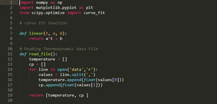
Step 1 :

Importing al the necessary libraries such as numpy, matplotlib.pyplot, scipy.optimize .

A function named linear is defined with the values of t, a, b.

A read_file function is used to Load the data of temperature and Specific heat capacity , an empty array is been created for the storages of their data.

(note: for the file to be read Data which is to be imported must be stored in the same current folder where the python coding is to be saved).

A for loop is been created so that at the each line data are splitted for both temperature and cp and furthermore the values are stored in append command.

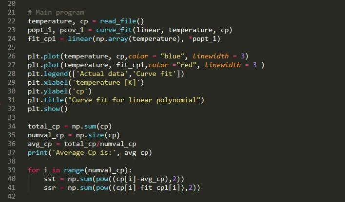
Step 2 :

Through data file , temperature and cp is taken. A popt and pocv is considered to make the curve fit into the arrays.

Fit_cp is been considered for linear function and this array is been taken individual arguments by using *popt.

plotting the temperature and cp curve results .

An average of cp values is been taken from total/numval, sst = total sum of squares and ssr = residual sum of squares is taken as a range function for cp and numval.

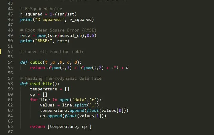
Step 3 :

Root mean square value is been calculated for numval_cp and ssr.

step 4 :

Same function is been defined but for cubic with values oft, a, b, c, d and the data of temperature and cp is taken from the read file data function.

now the floating values of temperature and cp are stored in append function.

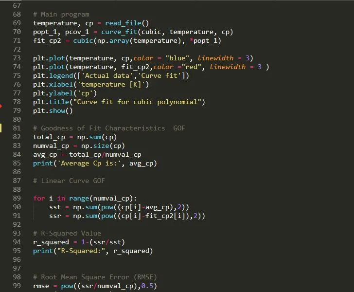
same all the plotting is been made like earlier for the cubic also.

Results:

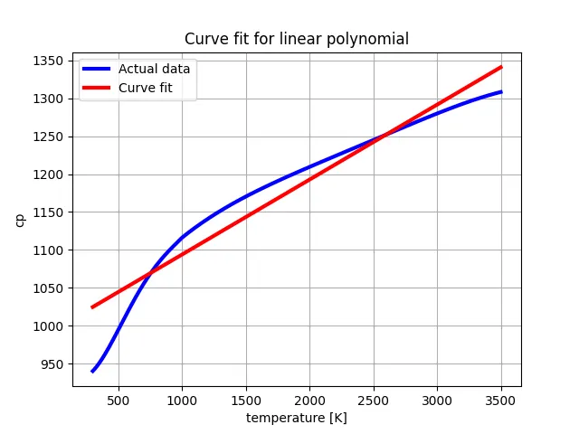
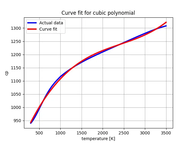
Result Discussion :

The analysis clearly shows that the cubic polynomial provides a significantly better fit to the Cp data than the linear model. With an R² of 0.98, the cubic model explains nearly all the variability in the data, making it a much more suitable model for this problem.

5. What needs to be done in order to make the curve fit perfect?

The degree of the polynomial should be adjusted to capture the data’s complexity. While higher-degree polynomials can improve the fit, they also risk overfitting, where the model captures noise instead of the actual trend. In such cases, cross-validation can help determine the optimal degree. Evaluating the goodness-of-fit metrics, such as R², RMSE, is vital for assessing the fit quality. A perfect fit ideally results in R²=1 and minimal error metrics. If the results are unsatisfactory, iterative refinement of the model, data preprocessing, or fitting strategy may be necessary.

6. Show empirically as to how well your curve has been fit.

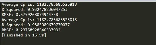
The cubic model explains 98% of the variance in the data, which is a significantly better fit than the linear model. The lower RMSE indicates that the cubic model more accurately predicts the actual ${\mathrm{\; cp\; values\; across\; the\; temperature\; range.}}_{}$

Linear Model: Although the linear model is easy to interpret and computationally efficient, it is not ideal for this dataset, as it fails to capture the full complexity of the temperature dependence of cp.

Cubic Model: The cubic model provides a much better fit, with a higher R² and lower RMSE, making it a more accurate representation of the relationship between temperature and cp.

metric	linear fit	cubic fit
R2	0.93	0.98
RMSE	0.575	0.237
Fit Quality	Moderate	Excellent

Conclusion :

The analysis clearly shows that the cubic polynomial provides a significantly better fit to the $C_p$Cp​ data than the linear model. With an $R^2$of 0.98, the cubic model explains nearly all the variability in the data, making it a much more suitable model for this problem.