Week 5 - Curve fitting
WEEK 5 - CURVE FITTING
ANSWERS
Question 1: What does popt and pcov mean? (Watch the video to get some context)

In Python, popt and pcov likely refer to variables typically used in the context of curve fitting or optimization problems, often encountered in libraries like scipy.optimize. Specifically:
a) popt: This typically stands for "optimized parameters." In the context of curve fitting or optimization, it refers to the set of parameters that minimizes or maximizes some objective function. For instance, in a curve fitting problem, popt would represent the optimized parameters of the curve that best fits the given data.
b) pcov: This typically stands for "covariance of parameters." It represents the estimated covariance of the optimized parameters (popt). Covariance gives you an idea of how two variables change together. In the context of curve fitting, it provides information about how uncertainties in the input data propagate to uncertainties in the optimized parameters.
In this example, popt contains the optimized parameters (slope and intercept) of the linear model that best fits the noisy data, while pcov contains the covariance matrix associated with these parameters.
Question 2 : What does np.array(temperature) do?
2) The "np.array(temperature)" command creates an array from the temperature values that were retrieved from the thermodynamic data file, using the "numpy" library. Having the temperature data in an array is useful in this code as it helps the code to calculate fitted "Cp" values for each respective temperature value based on the "popt" array.
Question 3: What does the * in *popt mean?
3) The "*" in the "*popt* tells the python code to indicate and return the values of the coefficients that are stored in the "popt" array.
in the context of *popt, if popt is a tuple or a list, *popt will unpack its elements wherever it's used.
This is often seen in functions that accept variable numbers of arguments or when you need to pass multiple arguments from a collection to a function.
Question 4: Python code for Linear fit Model
import math
import matplotlib.pyplot as plt
import numpy as np
from scipy.optimize import curve_fit
# Linear Fit Function, f(x) = ma + b
def linear_func(t, a, b):
return a*t + b
# Reading File
def read_file():
temperature = []
cp = []
for line in open('data', 'r'):
values = line.split(',')
temperature.append(float(values[0]))
cp.append(float(values[1]))
return [temperature, cp]
# Program for Linear fit
temperature, cp = read_file()
popt, pcov = curve_fit(linear_func, temperature, cp)
fit_cp1 = linear_func(np.array(temperature), *popt)
# Plots
plt.plot(temperature, cp, color = "blue", linewidth = 3)
plt.plot(temperature, fit_cp1, color = "red", linewidth = 3)
plt.legend(["Actual Data", "Linear Fit"])
plt.xlabel("Temperature [K]")
plt.ylabel("Cp")
plt.title("Linear fit Plot")
plt.show()
total_cp = np.sum(cp)
numval_cp = np.size(cp)
avg_cp = total_cp/numval_cp
print('Average Cp is:', avg_cp)
# GOF Characteristics
for i in range(numval_cp):
sst = np.sum(pow((cp[i]-avg_cp),2))
ssr = np.sum(pow((cp[i]-fit_cp1[i]),2))
# R-Squared Value
r_squared = 1-(ssr/sst)
print("R-Squared:", r_squared)
# Root Mean Square Error (RMSE)
rmse = pow((ssr/numval_cp),0.5)
print("RMSE:", rmse)
This Python code performs a linear fit on some data and evaluates the goodness of fit (GOF) characteristics, namely R-squared value and Root Mean Square Error (RMSE). Let's break down the code step by step:
a.Import necessary libraries:
- `math`: Provides mathematical functions.
- `matplotlib.pyplot`: Used for plotting.
- `numpy`: For numerical computing.
- `scipy.optimize.curve_fit`: Used to perform curve fitting.
b. Define a linear function:
This function represents a linear equation `f(t) = at + b`.
c. Define a function to read data from a file named `'data'`:
It reads temperature and Cp (specific heat capacity) values from a file where each line contains a temperature and Cp value separated by a comma. It returns two lists, one for temperature and one for Cp.
d. Perform linear fitting on the data:
It reads the data from the file using the `read_file()` function, then performs curve fitting using `curve_fit()` from `scipy.optimize`. The optimized parameters (`popt`) are used to generate fitted Cp values (`fit_cp1`).
e. Plot the actual data and the linear fit:
It plots the actual Cp values (`cp`) against temperature (`temperature`) in blue, and the linear fit in red.
f. Calculate the average Cp: It calculates the average Cp value.
g. Calculate R-squared value and RMSE:
It calculates the sum of squares total (SST) and sum of squares residual (SSR), and then uses these values to compute the R-squared value and RMSE, providing measures of how well the linear model fits the data.
Output:
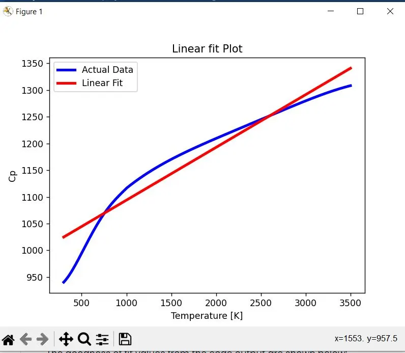
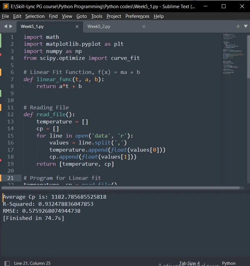
From this, we can see that the R-Squared value was 0.932 and the RMSE value was 0.576 to three decimal places. A valid measure of R-squared must always have a value between 0 and 1. The greater the goodness of fit for our model, the closer the number is to 1. Depending on the data set we are attempting to conduct the curve fit for, the RMSE value can also take any value. On the other hand, the goodness of fit increases with a decreasing RMSE value. In my instance, the RMSE value was quite low and the R-Squared value was very near to 1. These values indicated that the fitted linear model was reasonable. But as we can see from the graphical output, the linear model performs a poor job of simulating the actual data.
Python code for Cubic fit model
import math
import matplotlib.pyplot as plt
import numpy as np
from scipy.optimize import curve_fit
# Cubic Fit Function, f(x) = at^3 + bt^2 + ct+ d
def cubic_func(t, a, b, c, d):
return a*pow(t,3) + b*pow(t,2) + c*t + d
# Reading File
def read_file():
temperature = []
cp = []
for line in open('data', 'r'):
values = line.split(',')
temperature.append(float(values[0]))
cp.append(float(values[1]))
return [temperature, cp]
# Program for Cubic fit
temperature, cp = read_file()
popt, pcov = curve_fit(cubic_func, temperature, cp)
fit_cp1 = cubic_func(np.array(temperature), *popt)
# Plots
plt.plot(temperature, cp, color = "blue", linewidth = 3)
plt.plot(temperature, fit_cp1, color = "red", linewidth = 3)
plt.legend(["Actual Data", "Cubic Fit"])
plt.xlabel("Temperature [K]")
plt.ylabel("Cp")
plt.title("Cubic fit Plot")
plt.show()
total_cp = np.sum(cp)
numval_cp = np.size(cp)
avg_cp = total_cp/numval_cp
print('Average Cp is:', avg_cp)
# GOF Characteristics
for i in range(numval_cp):
sst = np.sum(pow((cp[i]-avg_cp),2))
ssr = np.sum(pow((cp[i]-fit_cp1[i]),2))
# R-Squared Value
r_squared = 1-(ssr/sst)
print("R-Squared:", r_squared)
# Root Mean Square Error (RMSE)
rmse = pow((ssr/numval_cp),0.5)
print("RMSE:", rmse)
Steps are same as previous Linear fit model. Only difference is the function
Define a Cubic function:
This function represents a linear equation ` f(t) = at^3 + bt^2 + ct+ d`.
Output
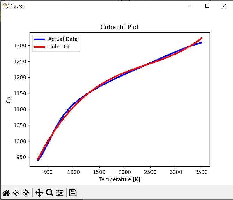
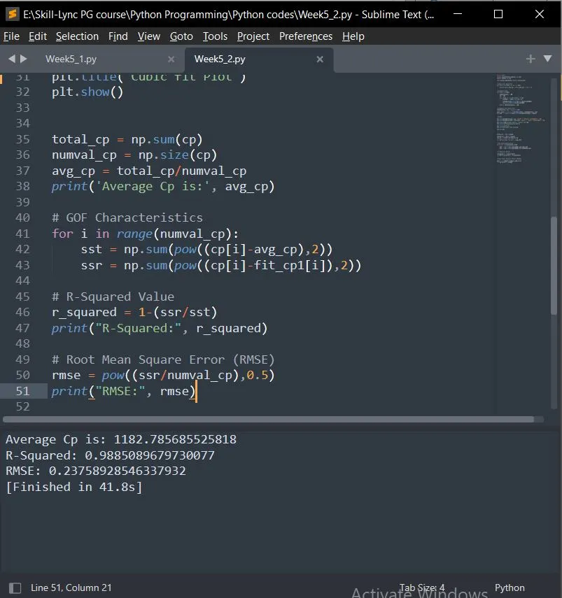
The R-Squared value was 0.989 and the RMSE value was 0.238 to three decimal places, according to the goodness of fit computations. The cubic model's RMSE value was lower and it was closer to a value of 1 than the linear model's R-Squared value. In this regard, the cubic model fits data better than the linear model. We can also observe from the graph output that the cubic model more closely matches the real data set. It is reasonable to conclude from these findings that the cubic model outperforms the linear model by a significant margin.
Question 5: What needs to be done in order to make the curve fit perfect?
Here are two methods to improve curve fit to the data.
- Adjusting the Fitted Function with Trial and Error:
- This method involves manually adjusting the coefficients of the fitted function (such as those in a polynomial equation) and observing the changes in the graphical output to determine if the fit improves.
- By trying different combinations of coefficients, you can explore a range of possible fits. However, this method can be time-consuming and subjective, especially when dealing with higher-dimensional models or complex functions.
- It's important to note that this method has limitations, particularly when using polynomial models. As you increase the order of the polynomial, there's a point where further increasing the order doesn't necessarily lead to a better fit and may even result in overfitting.
- Using Higher Order Polynomials:
- When the trial and error method reaches its limitations, using higher order polynomials can be beneficial.
- Higher order polynomials have more coefficients, which provide additional flexibility to adjust the shape of the curve to better match the data.
- By increasing the complexity of the model, higher order polynomials can capture more intricate patterns and variations in the data.
- However, it's essential to exercise caution with higher order polynomials as they can lead to overfitting, where the model fits the noise in the data rather than the underlying trend.
Question 6: Show empirically as to how well your curve has been fit.
It has been explained in the outputs and inference of Qn 4.