Week 5 - Curve fitting

Aim- To create plot of given data with curve fit of both linear and cubic equation and with splitting and find the goodness of curve by using R-square mathod.

Theory- Curve fitting is the process of making curve of any given data that fits the best on tat data , such that better analysis can be done on any study.

• python has an option of curve fit in the scipy library.
• popt- An array of optimal values for the parameters which minimizes the sum of squares of residuals.
• pcov-2d array which contains the estimated covariance of popt.
• np.array(Temperature) this command helps in giving all the values of temperature from the file that is 3200 values.
• Goodness of curve calculation is ised to determine the curve fit is having a good quality or bad quality, its is compared with 0-1 , if near to 0 the curve fit graph is bad and vice versa.

Results-

Case 1 - curve fitting is done by using a linear equation.

Python code-

#Importing modules
import numpy as np 
import matplotlib.pyplot as plt
import cmath
import math
from scipy.optimize import curve_fit

def read_file() :
	temperature = []
	cp = []
	for line in open('data','r') :
		values = line.split(',')
		temperature.append(float(values[0]))
		cp.append(float(values[1]))
	return[temperature,cp]
	
#Main program
temperature, cp = read_file()
#print(temperature)

#linear polynomial for curve fit
def func(t,a,b) :
	return a*t + b 


popt,pcov = curve_fit(func,temperature, cp)
#print(popt)
#print(pcov)
fit_cp = func(np.array(temperature), *popt)

# for plotting 
plt.plot(temperature, cp, color = 'red')
plt.plot(temperature,fit_cp, color = 'blue')
plt.xlabel('temperature')
plt.ylabel('cp')
plt.legend(['actual data','curve fit'])
plt.show()


# calculation of goodness of fit by using R-square method

A = np.power((np.array(np.array(cp)- np.array(fit_cp))),2)
SSE = np.sum(A)
B = np.mean(cp)
C = np.power(np.array((np.array(fit_cp)-B)),2)
SSR = np.sum(C)
SST = SSE+SSR
R_Square = SSR/SST
print(R_Square)

graph of case 1 -

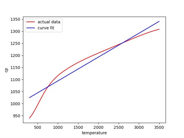
In case 1 the goodness of curve value is - 0.9248776260524184

Case 2 - Curve fitting is done by using a cubic equation-

Python code-

#Importing modules
import numpy as np 
import matplotlib.pyplot as plt
import cmath
import math
from scipy.optimize import curve_fit

def read_file() :
	temperature = []
	cp = []
	for line in open('data','r') :
		values = line.split(',')
		temperature.append(float(values[0]))
		cp.append(float(values[1]))
	return[temperature,cp]
	

#cubic polynomial for curve fit
def func(t,a,b,c,d) :
	return a*np.power(t,3)+b*np.power(t,2)+c*t+d 

#Main program
temperature, cp = read_file()
#print(temperature)

popt,pcov = curve_fit(func,temperature, cp)
#print(popt)
#print(pcov)
fit_cp = func(np.array(temperature), *popt)

# for plotting 
plt.plot(temperature, cp, color = 'red')
plt.plot(temperature,fit_cp, color = 'blue')
plt.xlabel('temperature')
plt.ylabel('cp')
plt.legend(['actual data','curve fit'])
plt.show()

# calculation of goodness of fit by using R-square method

A = np.power((np.array(np.array(cp)- np.array(fit_cp))),2)
SSE = np.sum(A)
B = np.mean(cp)
C = np.power(np.array((np.array(fit_cp)-B)),2)
SSR = np.sum(C)
SST = SSE+SSR
R_Square = SSR/SST
print(R_Square)

graph of case 2 -

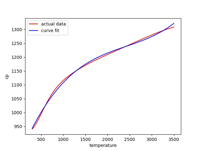
The goodness of curve value in this case is - 0.9967259467146888

Case 3 - curve fitting is done by splitting in range of temperature and cp parameters which is done on two parts - first one is - 0-1600 values and second one is 1601 -3200 values .

python code-

#Importing modules
import numpy as np 
import matplotlib.pyplot as plt
import cmath
import math
from scipy.optimize import curve_fit


def read_file() :
	temperature = [] #Range 1 
	cp = []
	for line in open('data','r') :
		values = line.split(',')
		temperature.append(float(values[0]))
		cp.append(float(values[1]))
	return[temperature,cp]
temperature, cp = read_file()


# Splitting data
# Range 1 
temperature1 = np.array(temperature[0:1600])
cp1 = np.array(cp[0:1600])

#linear polynomial for curve fit
def func(t,a,b) :
	return a*t + b 

popt,pcov = curve_fit(func,temperature1, cp1)
#print(popt)
#print(pcov)
fit_cp1 = func(np.array(temperature1), *popt)

# for plotting 
plt.plot(temperature1, cp1, color = 'red')
plt.plot(temperature1,fit_cp1, color = 'blue')
plt.xlabel('temperature')
plt.ylabel('cp')
plt.legend(['actual data','curve fit'])
plt.show()

# calculation of goodness of fit by using R-square method

A = np.power((np.array(np.array(cp1)- np.array(fit_cp1))),2)
SSE = np.sum(A)
B = np.mean(cp)
C = np.power(np.array((np.array(fit_cp1)-B)),2)
SSR = np.sum(C)
SST = SSE+SSR
R_Square = SSR/SST
print(R_Square)




# For range 2

# Splitting data
# Range 2 
temperature2 = np.array(temperature[1601:3200])
cp2 = np.array(cp[1601:3200])

#cubic polynomial for curve fit

def func(t,a,b,c,d) :
	return a*pow(t,3)+b*np.power(t,2)+c*t+d 

popt,pcov = curve_fit(func,temperature2, cp2)
#print(popt)
#print(pcov)
fit_cp2 = func(np.array(temperature2), *popt)

# for plotting 
plt.plot(temperature2, cp2, color = 'red')
plt.plot(temperature2,fit_cp2, color = 'black')
plt.xlabel('temperature')
plt.ylabel('cp')
plt.legend(['actual data','curve fit'])
plt.show()

# calculation of goodness of fit by using R-square method

A = np.power((np.array(np.array(cp2)- np.array(fit_cp2))),2)
SSE = np.sum(A)
B = np.mean(cp)
C = np.power(np.array((np.array(fit_cp2)-B)),2)
SSR = np.sum(C)
SST = SSE+SSR
R_Square = SSR/SST
print(R_Square)

graph of case 3 part 1 (0-1600)

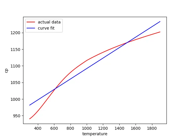
here the range is from 0-1600 and the value of goodness of curve is -0.9659874514138078

Case 3 part 2 (1601-3200) graph

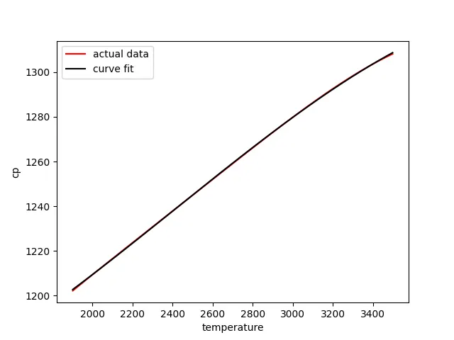
here the cubic equation is conssidered and the value of goodness of curve is - 0.9999951618140007.

It is observed that the goodness of curve is more when the cubic equation is considered. As the actual graph is behaving like a cubic equation.