Week 5 - Curve fitting

Introduction

Curve fitting

For root finding, we used a given function to identify where it crossed zero, capturing the data trend by assigning a single function across the entire range.

mathematically

General

`f(x)=ax+b` 

The goal is to identify the coefficients ‘a’ and ‘b’ such that f(x) ‘fits’ the data well

polynomial (for higher oders)

`f(x)=a_0+a_1x+a_2x^2+a_3x^3...+a_jx^j=a_0+sum_(k=1)^ja_kx^k`

python code

"""
CURVE FITTING BY JAGAVEERAPANDIYAN.S
"""
import numpy as np
import matplotlib.pyplot as plt
from scipy.optimize import curve_fit

#first Degree of polynomial
def fun(t,a,b):
	return a*t + b

# reading Thermodynamic property
def read_file():
	temperature = []
	cp = []
	for line in open('data','r'):
		values = line.split(',')
		temperature.append(float(values[0]))
		cp.append(float(values[1]))

	return [temperature, cp]

temperature, cp = read_file()
popt , pcov = curve_fit(fun,temperature,cp)
fit_cp = fun(np.array(temperature), *popt)

print(popt)


#secound Degree of polynomial
def funs(t,a,b,c):
	return a*pow(t,2) + b*t + c

# reading Thermodynamic property
def read_file():
	temperatures = []
	cps = []
	for line in open('data','r'):
		values = line.split(',')
		temperatures.append(float(values[0]))
		cps.append(float(values[1]))

	return [temperatures, cps]

temperatures, cps = read_file()
popt , pcov = curve_fit(funs,temperatures,cps)
fit_cps = funs(np.array(temperatures), *popt)

print(popt)

plt.figure(1)
plt.plot(temperature,cp,color="blue",linewidth=3)
plt.plot(temperature,fit_cps,"k",linewidth=1)
plt.plot(temperature,fit_cp,"r--",linewidth=1)
plt.legend(['Actual data','secound degree curve fit','first degree curve fit'])
plt.xlabel('Temperature [k]')
plt.ylabel('cp (j/khk')
plt.title('curve fit for T vs cp ')
plt.grid()
plt.show()


# cubic polynomial fit function 
def func(t,a,b,c,d):
	return a*pow(t,3) + b*pow(t,2) + c*t+d

#read the data file provided
def read_file():
	temperaturec=[]
	cpc=[]
	for line in open('data','r'):
		values = line.split(',')
		temperaturec.append(float(values[0]))
		cpc.append(float(values[1]))

	return [temperaturec, cpc]

temperaturec, cpc = read_file()
popt , pcov = curve_fit(func,temperaturec,cpc)
fit_cpc = func(np.array(temperaturec), *popt)

print(popt)

# fourth polynomial fit function 
def funf(t,a,b,c,d,e):
	return a*pow(t,4) + b*pow(t,3) + c*pow(t,2)+d*t+e

#read the data file provided
def read_file():
	temperaturef=[]
	cpf=[]
	for line in open('data','r'):
		values = line.split(',')
		temperaturef.append(float(values[0]))
		cpf.append(float(values[1]))

	return [temperaturef, cpf]

temperaturef, cpf = read_file()
popt , pcov = curve_fit(funf,temperaturef,cpf)
fit_cpf = funf(np.array(temperaturef), *popt)

print(popt)

plt.figure(2)
plt.plot(temperature,cp,"b",linewidth=3)
plt.plot(temperature,fit_cp,"k",linewidth=1)
plt.plot(temperature,fit_cps,"r--",linewidth=1)
plt.plot(temperature,fit_cpc,"g-.",linewidth=1)
plt.plot(temperature,fit_cpf,"y-",linewidth=1)
plt.legend(['Actual data','curve fit first','curve fit secound','curve fit cubic','curve fit fouth'])
plt.xlabel('Temperature [k]')
plt.ylabel('cp (j/khk')
plt.title('curve fit comparison for T vs cp ')
plt.grid()
plt.show()

 code Procedure

import the external note file by reading the file & open file split using split command at ',' and save as floating values.

use popt and pcov curve_fit function (polynomials expression) & inputs to get curve fit values of cp

stored the curve fit data in variables

popt : array

Optimal values for the parameters so that the sum of the squared error of f(xdata, *popt) - ydata is minimized

pcov : 2d array

The estimated covariance of popt. The diagonals provide the variance of the parameter estimate. To compute one standard deviation errors on the parameters use perr = np.sqrt(np.diag(pcov)).

How the sigma parameter affects the estimated covariance depends on the absolute sigma argument, as described above.

np.array(temperature)

storing temperature variable in the array 

* in *popt

 function again to fit the curve taking the temperature value from the array and a,b,c etc variable (*popt) * use the value a,b,c etc stored in popt and then use them while plotting

plot the result and compare the result with actual data

Plot

First & secound

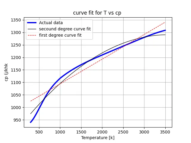
 the first order is taken polynomial a,b constant in second order polynomial a,b,c constant increases here the level of accuracy near to real data some what good than first oder

Cubic & higher order

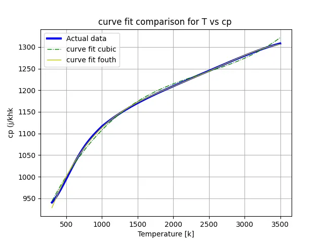
cubic polynomial which is approximately approaching real-time data with a lesser variable so it calculates faster. if there is precious result demand fourth order is better by the polynomial will be more so solving can take time

comparison of all

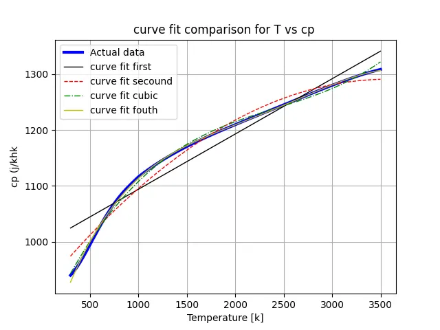
Getting the curve fit perfectly

reduce the error by increasing the order of polynomial which perfectly fit actual data, or split wise polynomial give accurate result ( split the solution)

conclusion

By increasing the order of polynomial we will get an accuracy of the result by reducing data noise (error)

References

https://docs.scipy.org/doc/scipy-0.15.1/reference/generated/scipy.optimize.curve_fit.html

https://en.wikipedia.org/wiki/Curve_fitting